Introduction
High-quality astronomical images delivered by modern ground-based and space observatories demand adequate, reliable software for
their analysis and accurate extraction of sources, filaments, and other structures, containing massive amounts of detailed
information about the complex physical processes in space. The multi-wavelength observations with highly variable angular
resolutions across wavebands require extraction tools that preserve and use the invaluable high-resolution information. Complex
fluctuating backgrounds and filamentary structures appear differently on various scales, calling for multi-scale approaches for
complete and reliable detection of sources and filaments. Availability of uncalibrated extraction tools with widely varying
qualities highlights the need to use standard benchmarks for choosing the most reliable and accurate method for the astrophysical
research.
These pages present getsf, a new method for extracting sources and filaments in
astronomical images using separation of their structural components, designed to handle multi-wavelength sets of images and very
complex filamentary backgrounds. The method spatially decomposes the original images and separates the structural components of
sources and filaments from each other and from their backgrounds, flattening their resulting images. It spatially decomposes the
flattened components, combines them over wavelengths, and detects the positions of sources and skeletons of filaments. Finally,
getsf measures the detected sources and filaments and creates the output catalogs
and images. This almost universal and fully automated method has a single user-definable parameter, the maximum size of the
structures to extract, that users have to determine from the input images on the basis of their research interests.
These pages describe a realistic multi-wavelength set of benchmark images for testing and comparing source and filament extraction
methods to enable the selection of the most reliable and accurate method. The images include a complex fluctuating background
cloud, a long dense filament, and many starless and protostellar cores. The benchmark enables conclusive comparisons according to
the extraction completeness, reliability, and goodness, as well as the detection and measurement accuracies and the overall quality.
Multi-wavelength source and filament extractions with getsf using three variants of
the new benchmark with increasing complexity levels show that the new method is superior to older methods.
An improved algorithm for the derivation of high-resolution surface density images from the multi-wavelength far-infrared and
submillimeter continuum imaging is shown to create the densities as sharp as the shortest-wavelength image of a sufficient quality,
with the angular resolution reaching 5.6" when using the Herschel
70 μm image. If the image is excessively noisy, contaminated by the PAH emission, or unusable
for other reasons, the highest resolution is defined by the 100 or
160 μm images
(6.8–11.3"). Such high resolution is useful for
detailed studies of the enormous structural diversity in space, hence, for deeper understanding of the physical processes within
the sub-structured filaments and their relation to the formation of stars.
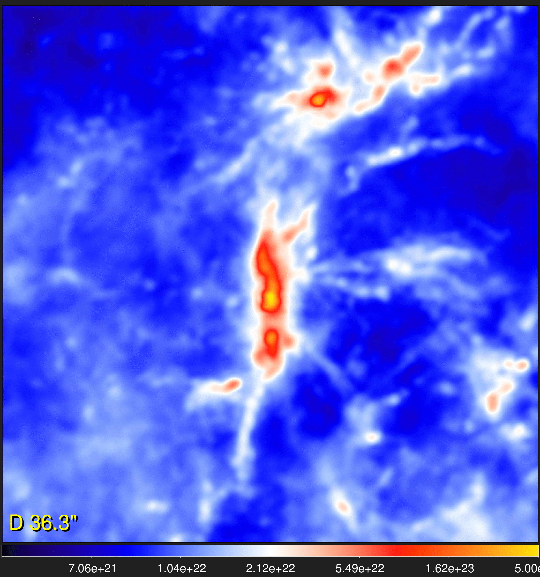
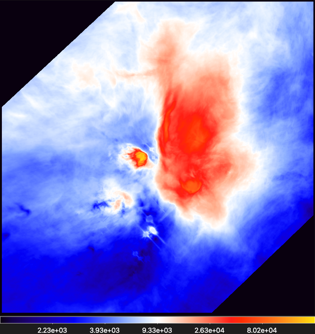
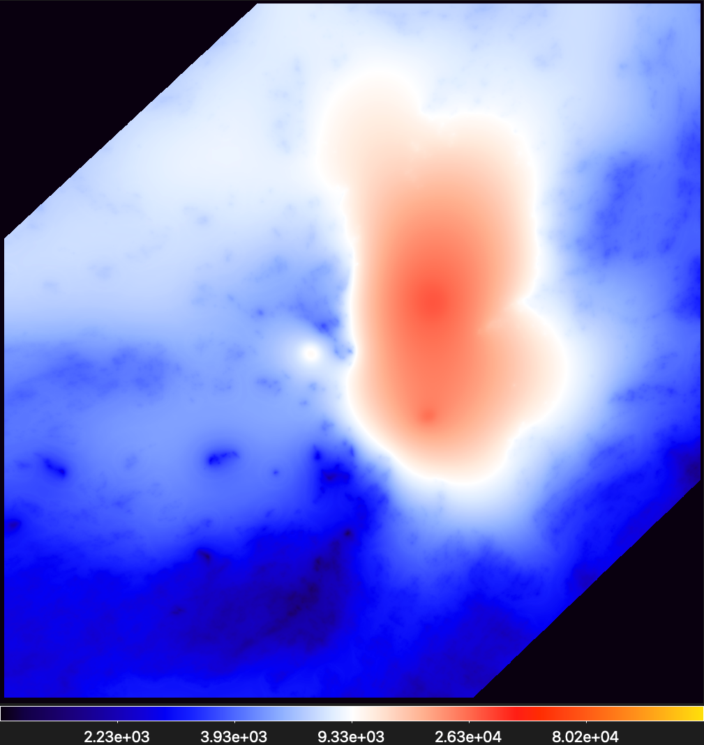
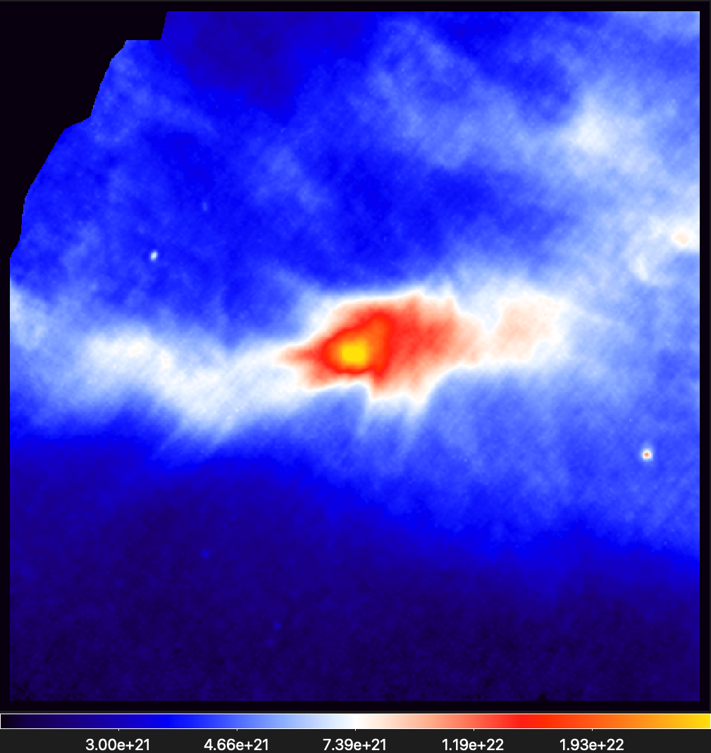
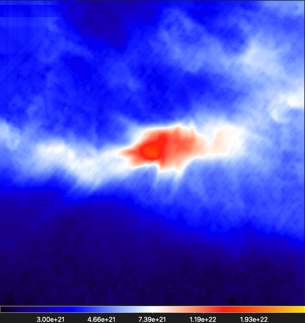
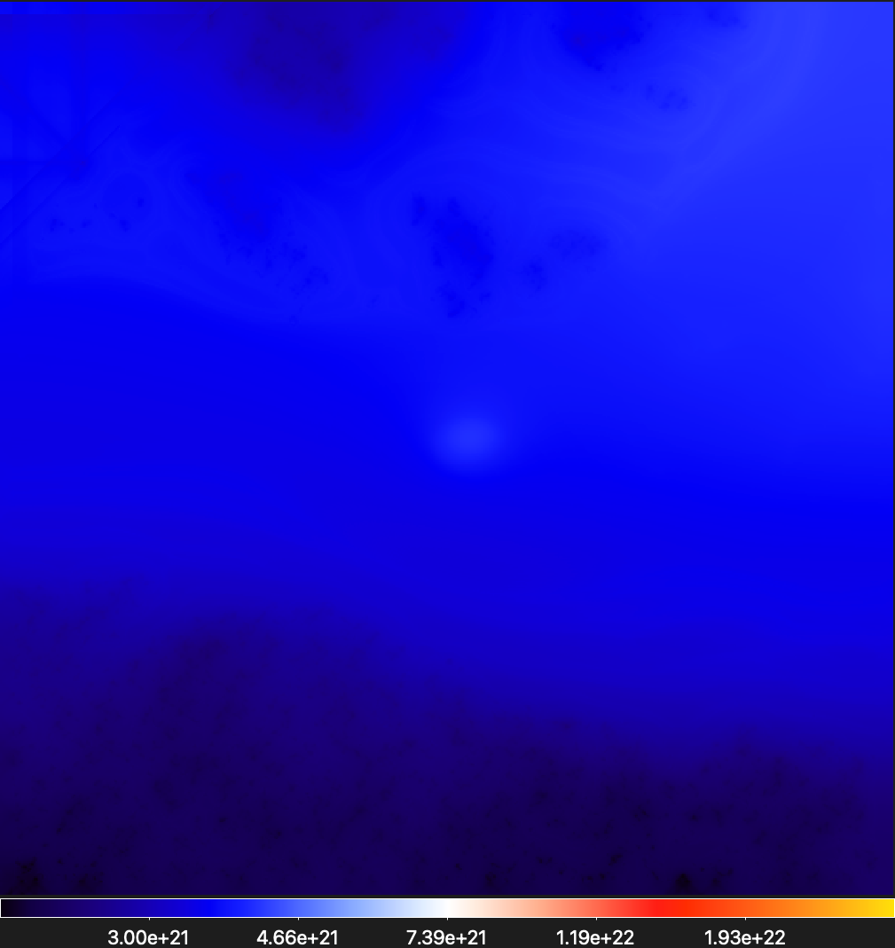
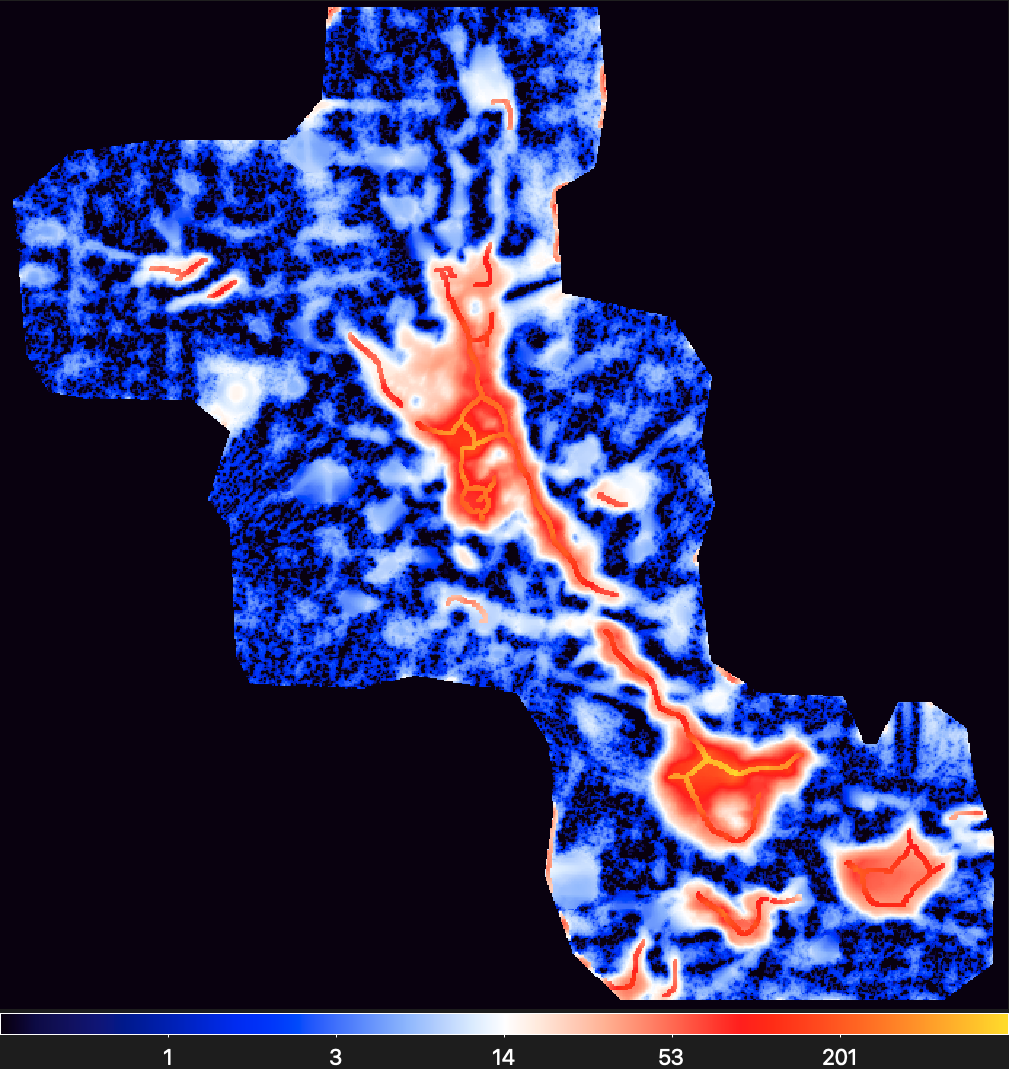
Star-Forming Cloud DR21 (Cyg X)
Illustration of the new algorithm for the derivation of high-resolution surface densities from multi-wavelength observations.
The density was derived from 5 images (at 70–500 μm)
obtained with the Herschel Space Observatory (Motte et al. 2010;
Hennemann et al. 2012; Bontemps et al., in prep.).
High-res surface density (36.3, 24.9,
18.2, 11.7,
5.9")
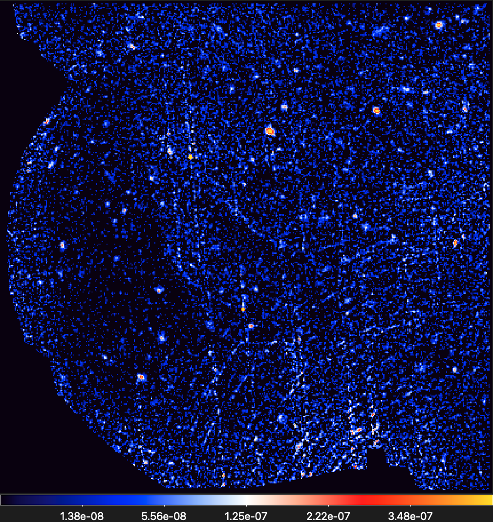
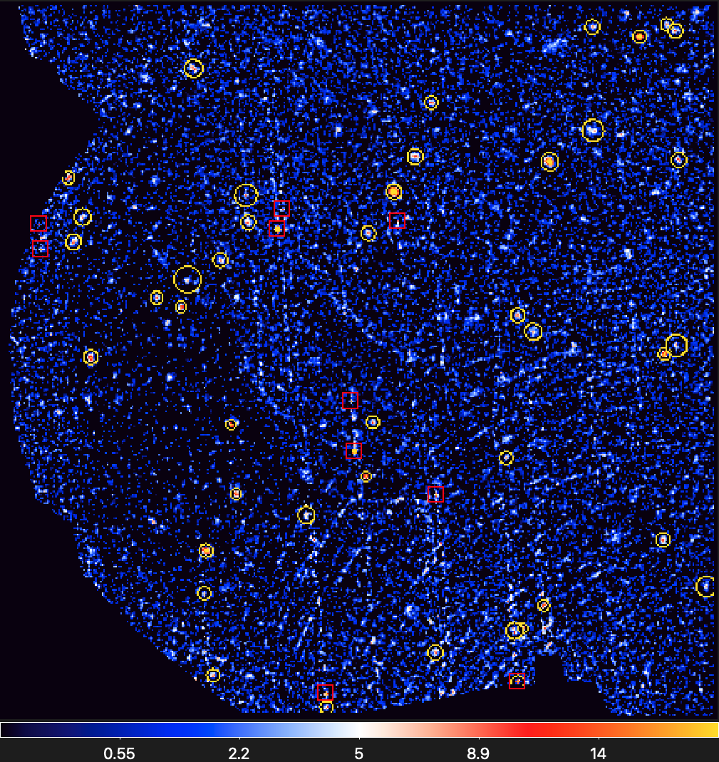
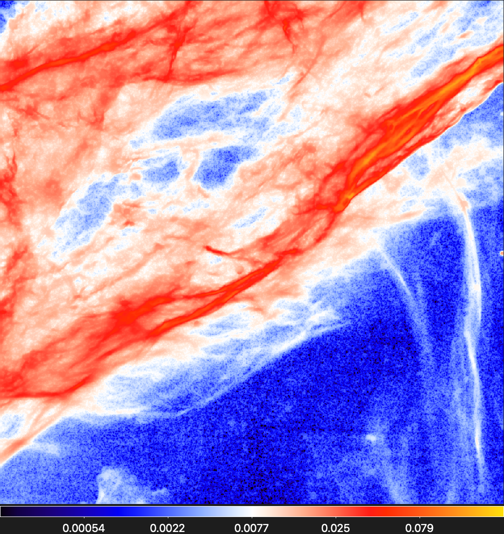
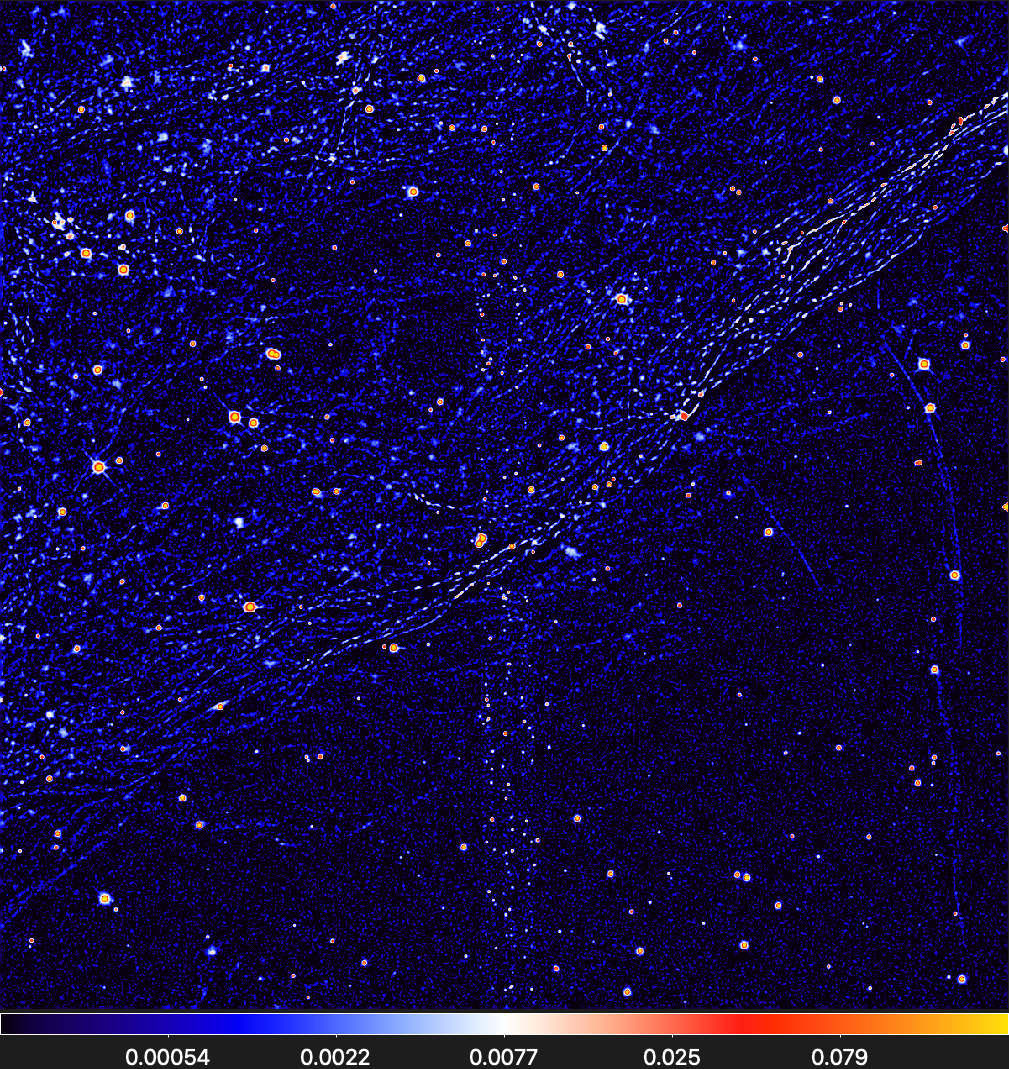
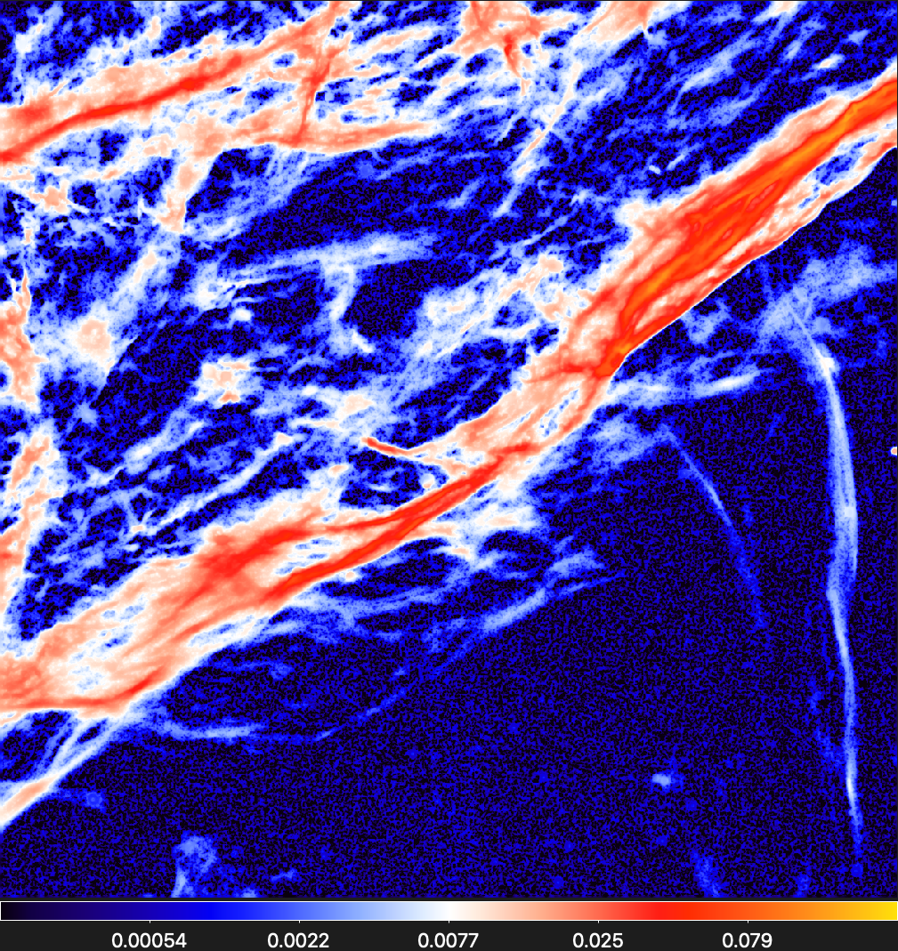
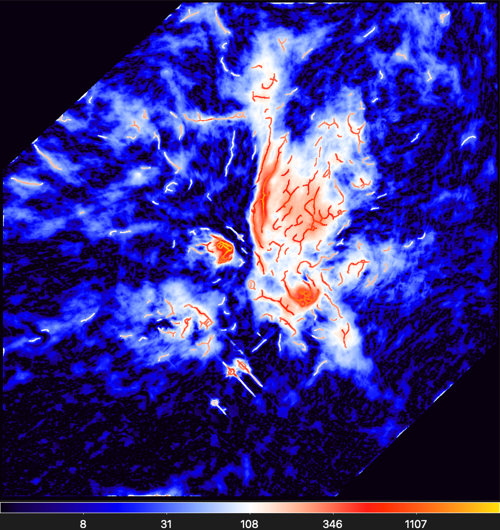
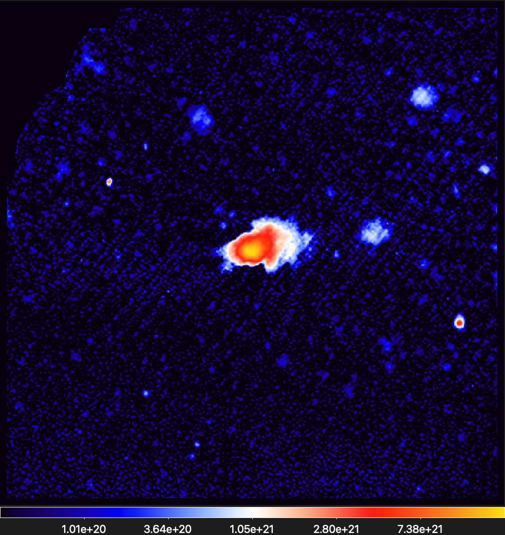
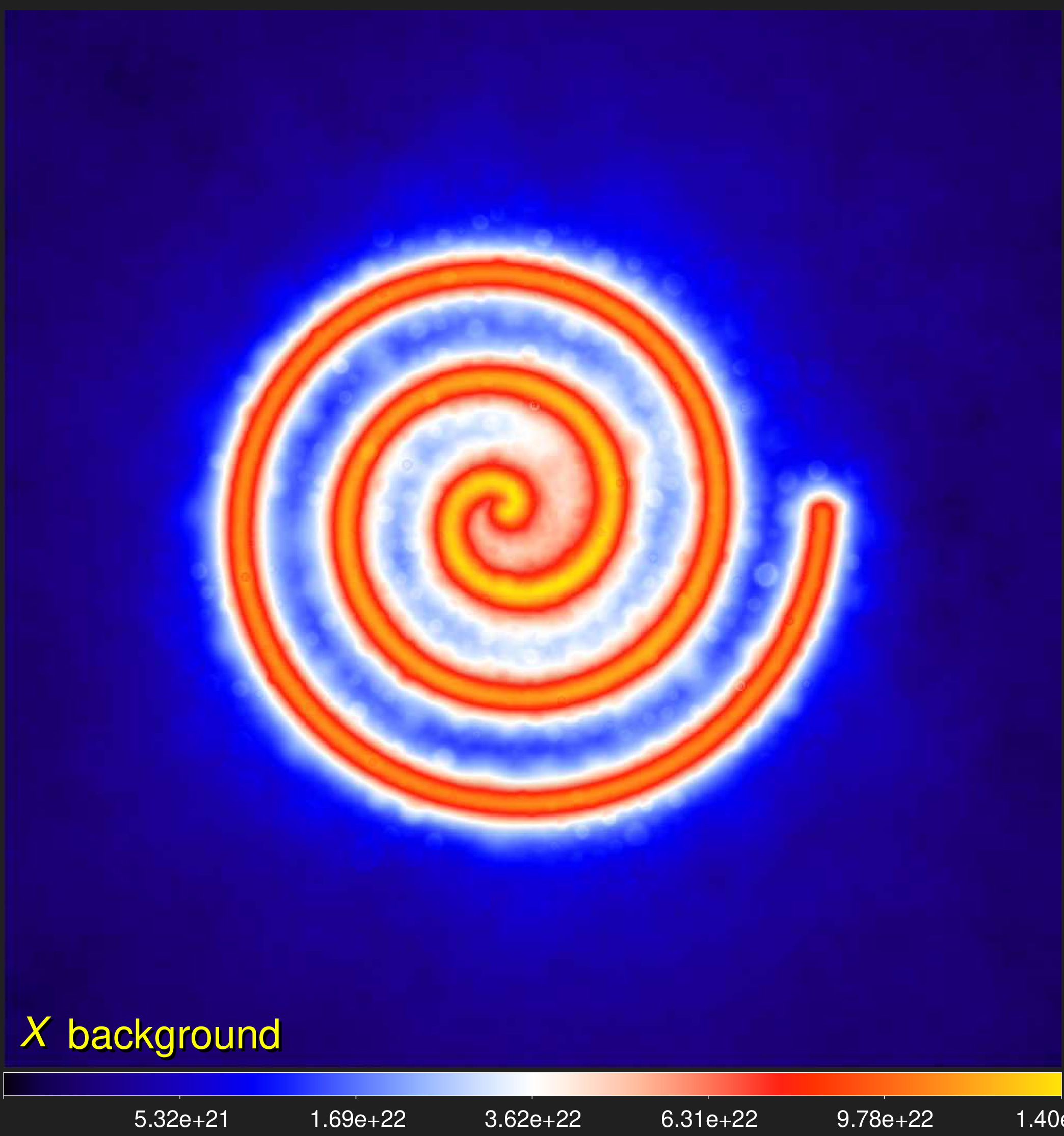
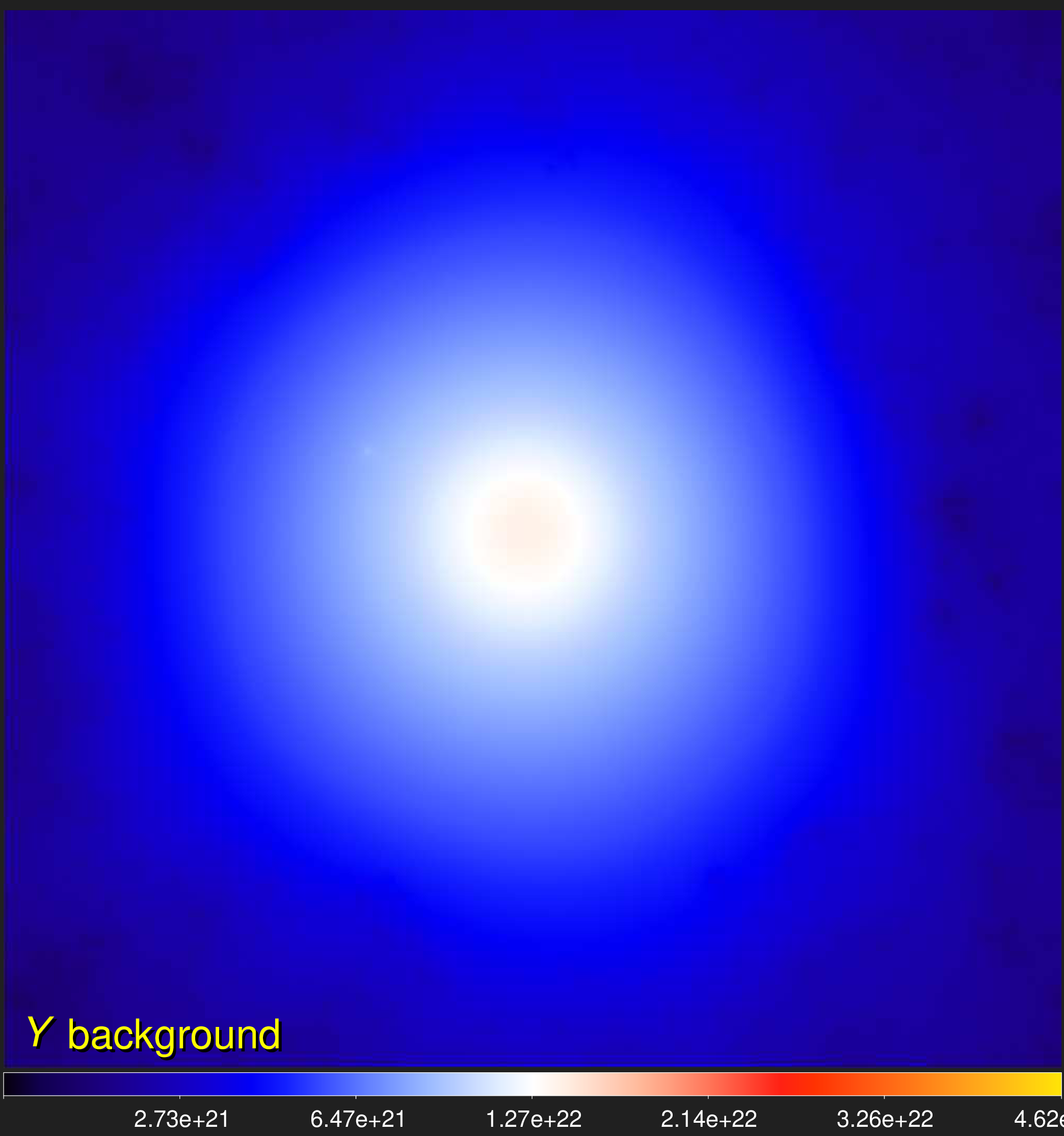
Supernova Remnant RXJ1713.7-3946
RXJ1713.7-3946 was observed with XMM-Newton (EPIC camera) in the X-ray waveband
(0.6–6 keV) centered at
0.0024 μm. The image below is a mosaic of multiple
observations, first presented in
Acero et al. (2017). With an average angular resolution of
7", it reveals the south-east segment of the supernova remnant shell, possibly
created by the explosion of the historical supernova SN393, whose center of explosion is located beyond the upper-right image
corner. For this source and filament extraction with getsf, a maximum size of
15" of the sources and 25" of the filaments of interest
was adopted.
XMM-Newton (EPIC) image at 0.0024 microns
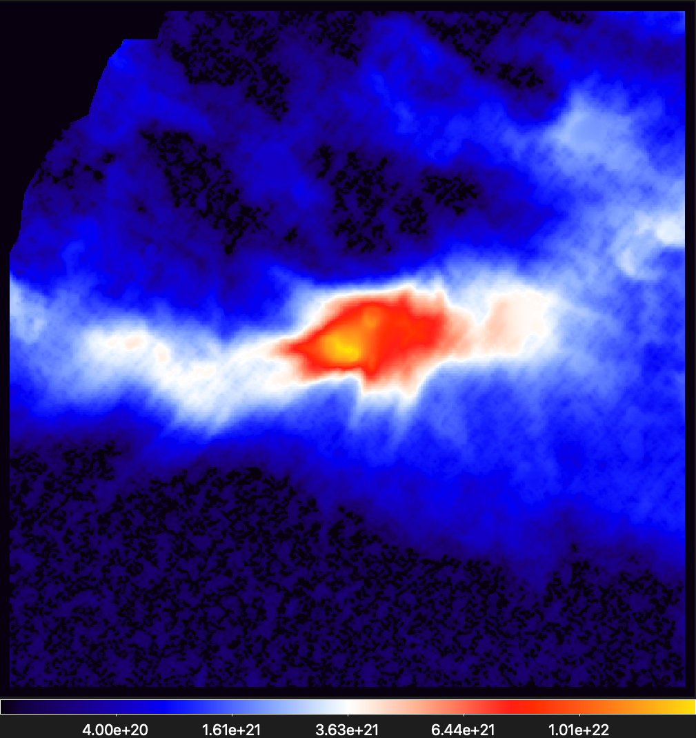
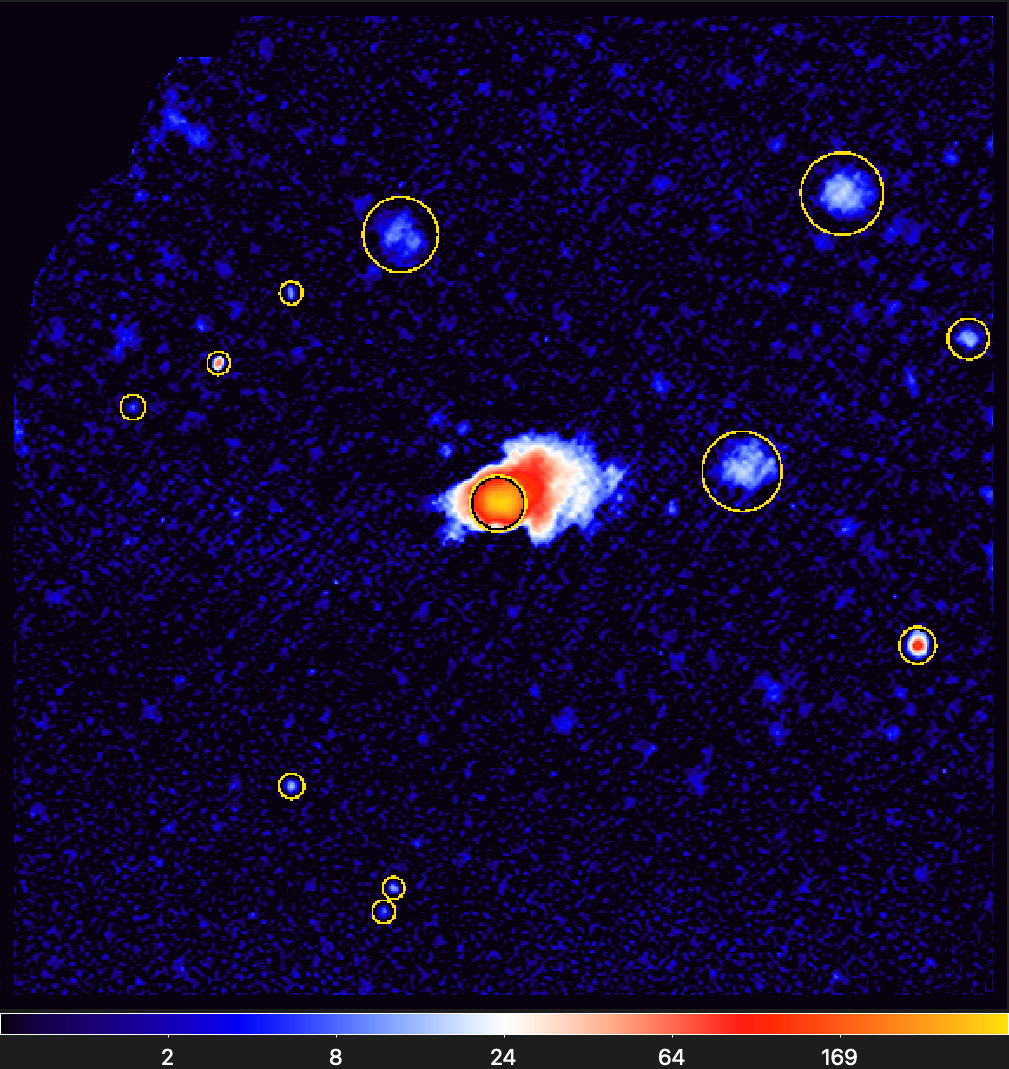
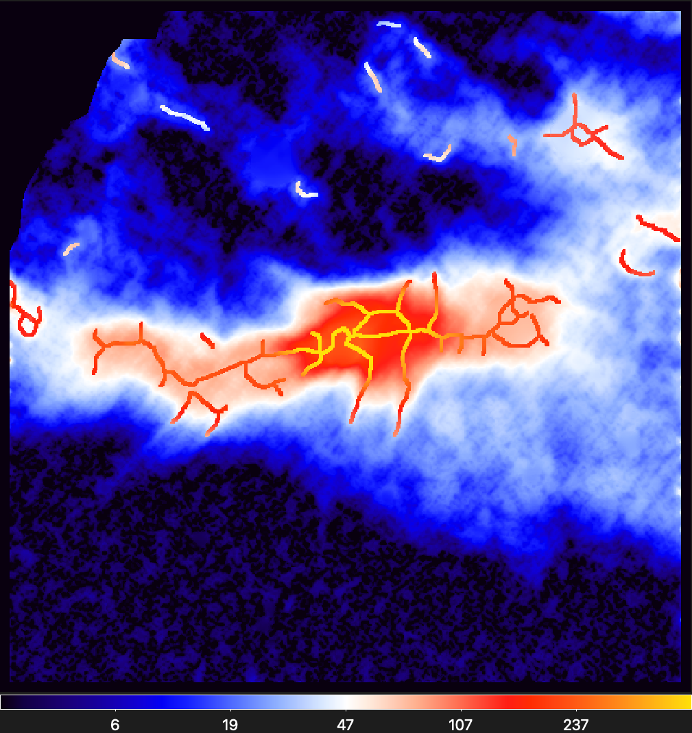
Background of sources
Background of filaments
Component of sources
Component of filaments
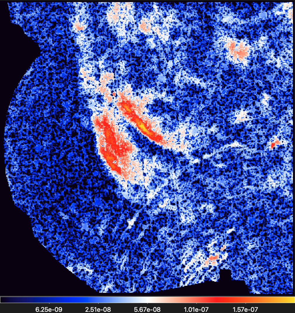
Extracted sources (footprints)
Extracted filaments (skeletons on scales 7–25")
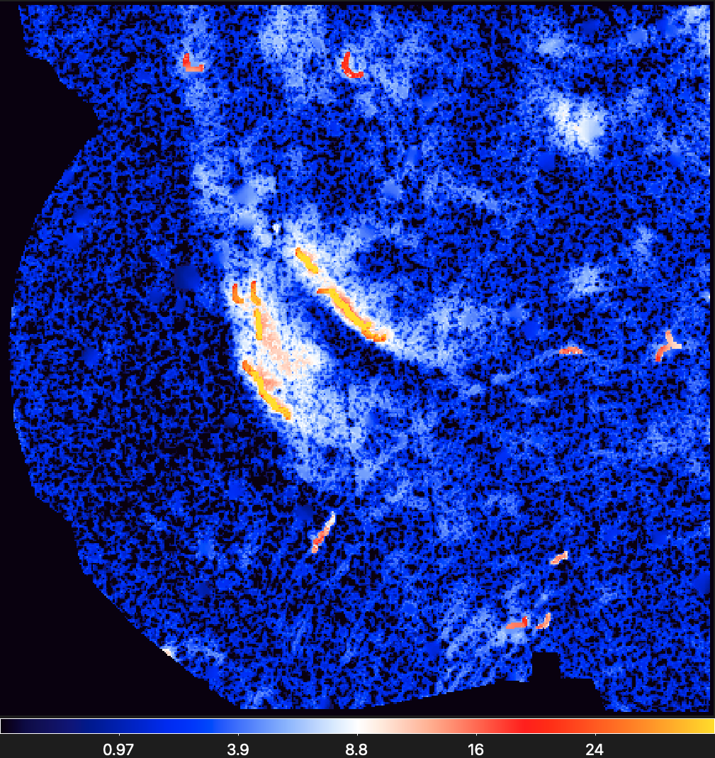
Extracted filaments (skeletons on scales ~28")

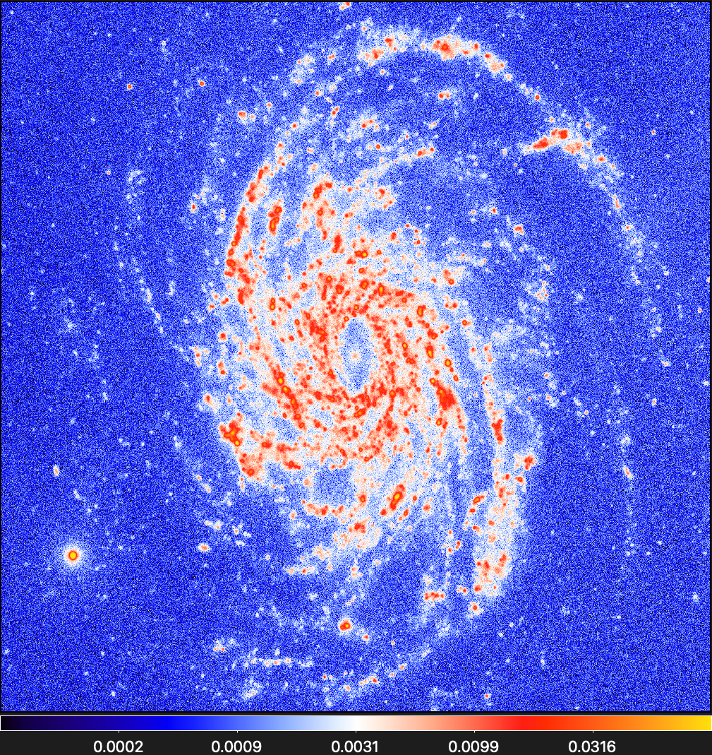
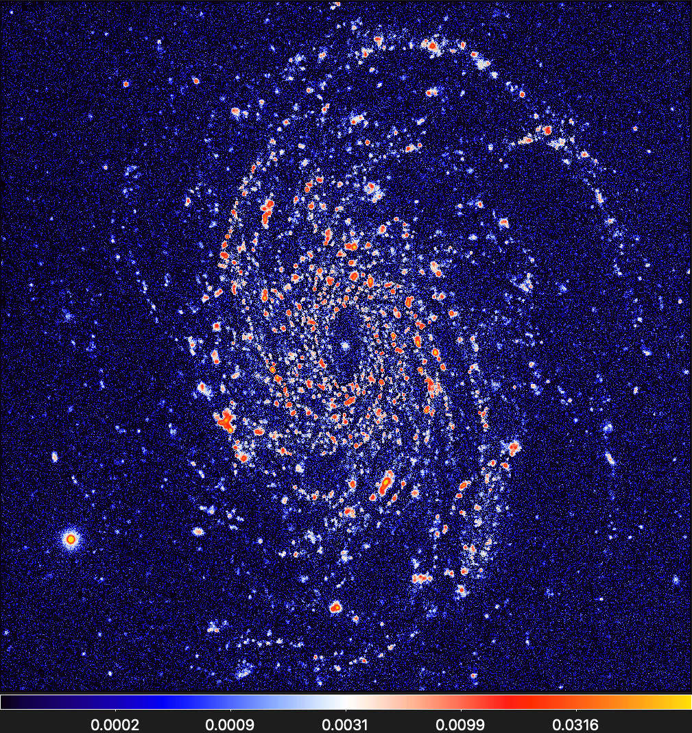
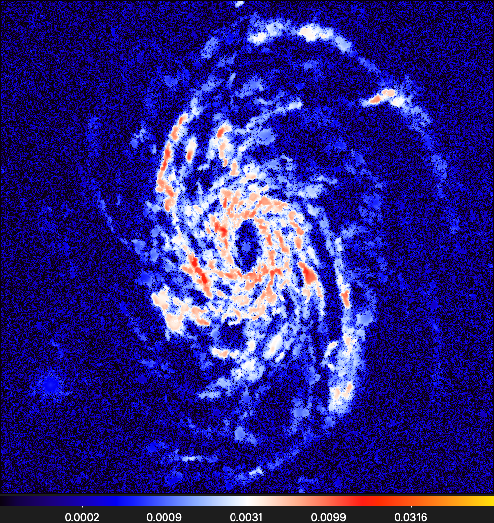
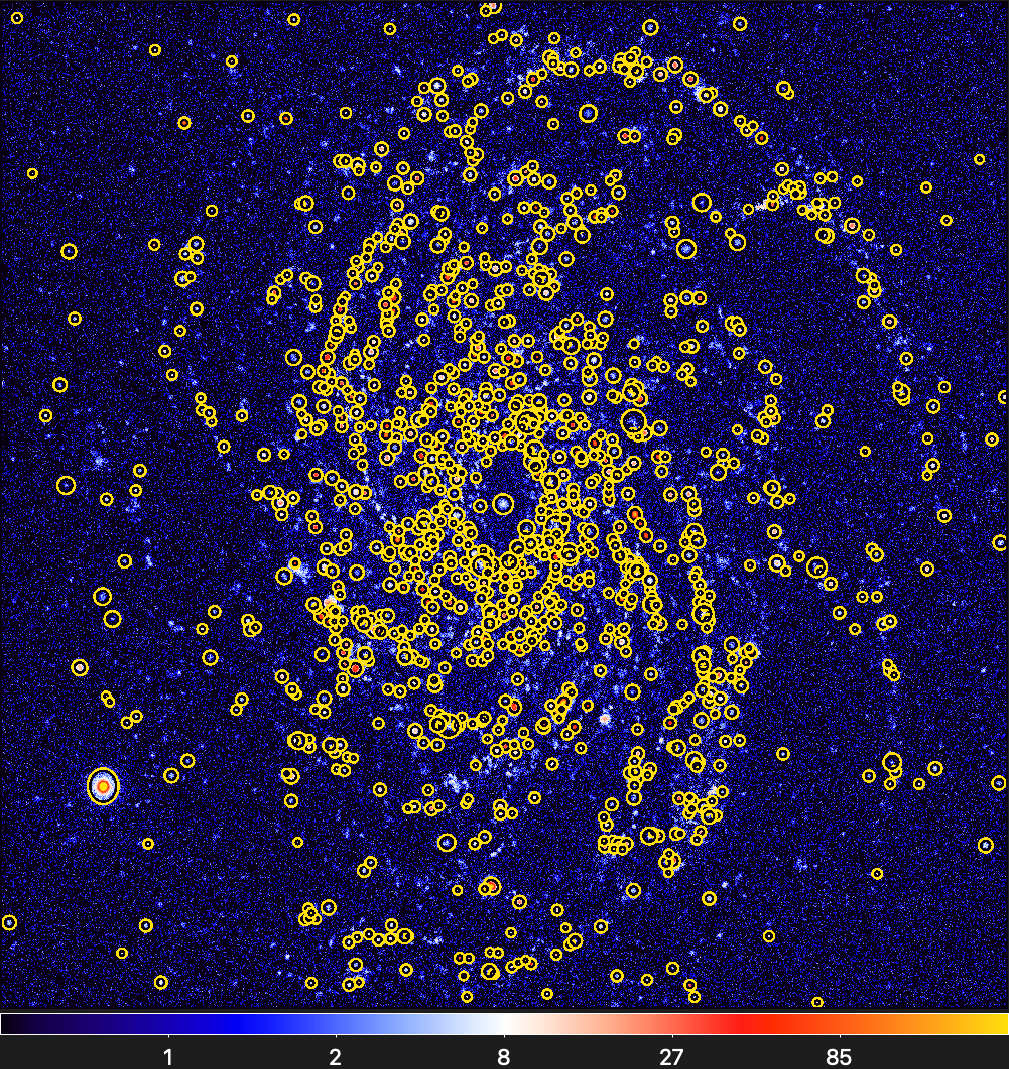
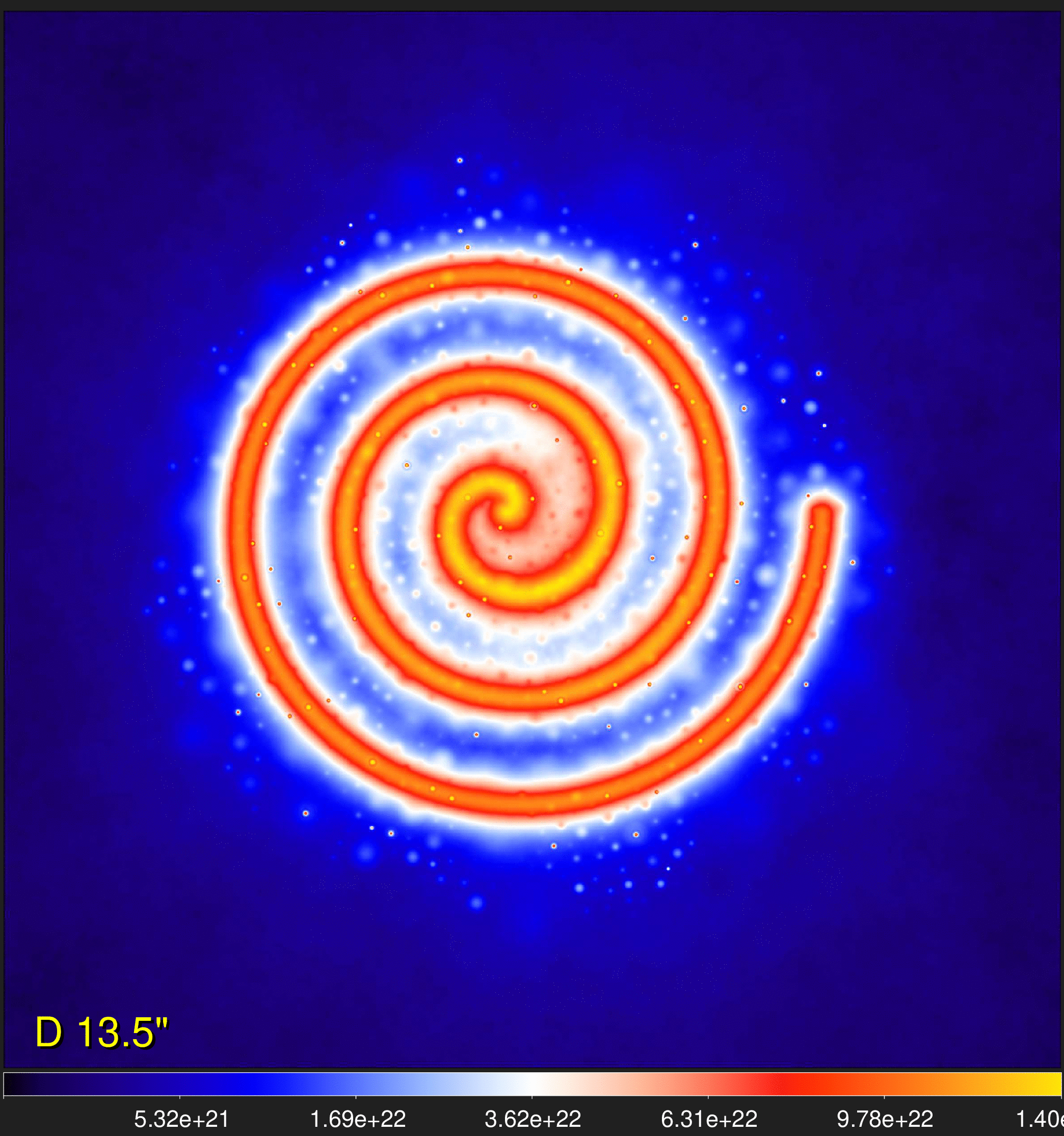
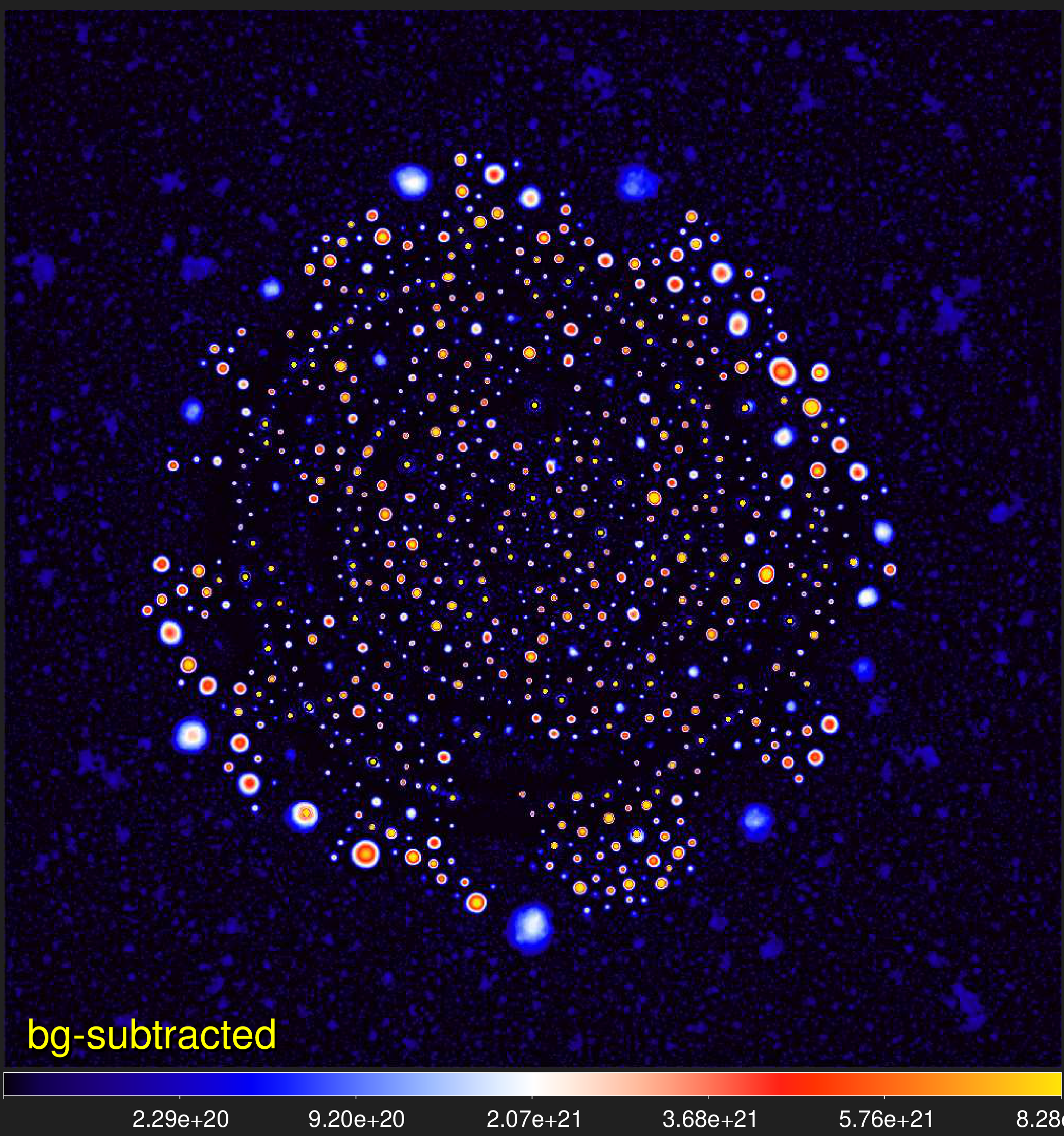
Star-Forming Galaxy NGC6744
NGC6744 was observed with GALEX in a far-ultraviolet (FUV) waveband
(1350–1750 Å) centered at
0.15 μm (Lee et al. 2011). The
image below with an angular resolution of
4" shows the spiral galaxy, considered similar to our own Galaxy. Despite noisiness of
the FUV image, it displays the spiral arms with many hundreds of unresolved emission sources – the regions of ongoing
star formation, heated by the embedded young massive stars. For this source and filament extraction with
getsf, a maximum size of 20" of the sources
and filaments of interest was adopted.
GALEX (FUV) image at 0.15 microns
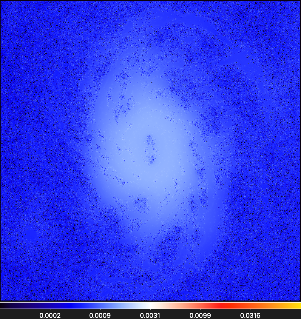
Background of sources
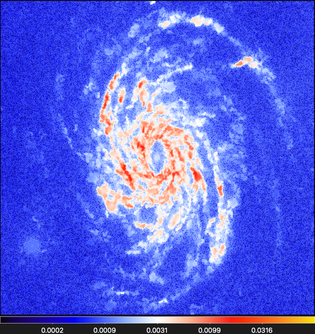
Background of filaments
Component of sources
Component of filaments
Extracted sources (footprints)
Extracted filaments (skeletons on scales 4–20")
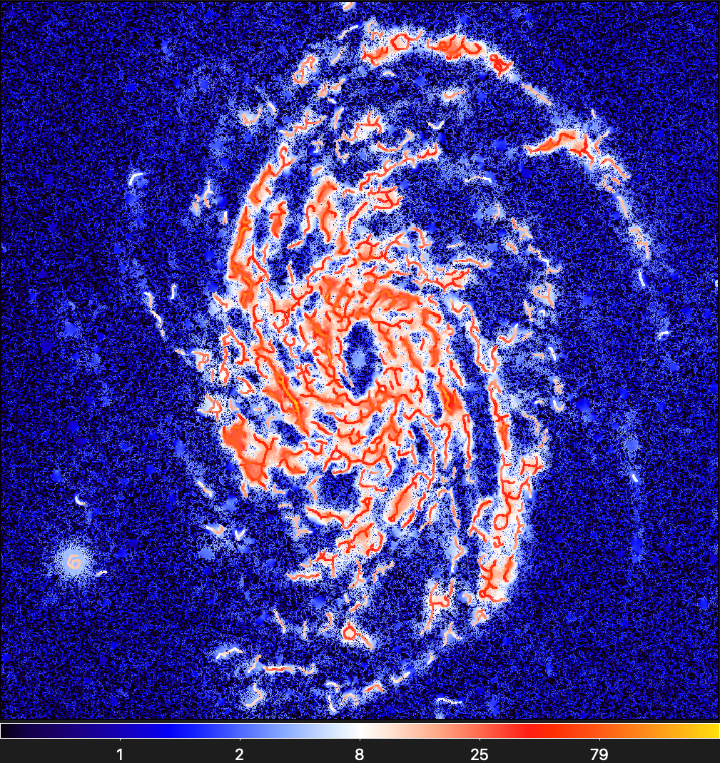
Extracted filaments (skeletons on scales ~20")

Supernova Remnant NGC6960
NGC6960 was observed with Hubble in five UVIS wavebands
(0.5–0.8 nm) centered at
0.6 μm, within the frame of the Hubble Heritage project (PI: Z. Levay;
Mack et al. 2015). The small
image below with an angular resolution of
0.2" represents a small fragment of the Veil Nebula, which is a segment of the Cygnus Loop, the
large expanding shell of a supernova remnant (Fesen et al. 2018). For this source and filament extraction with
getsf, a maximum size of 0.5" of the
sources and 2" of the filaments of interest was adopted.
Hubble (WFC3) image at 0.6 microns
Background of sources
Background of filaments
Component of sources
Component of filaments
Extracted sources (footprints)
Component of filaments (skeletons on scales 0.2–2")
Component of filaments (skeletons on scales ~2")

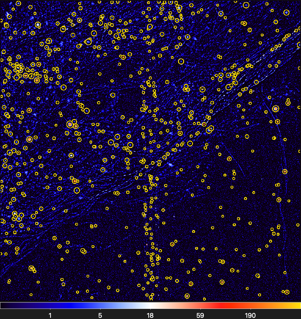
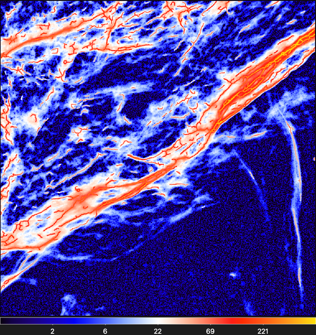
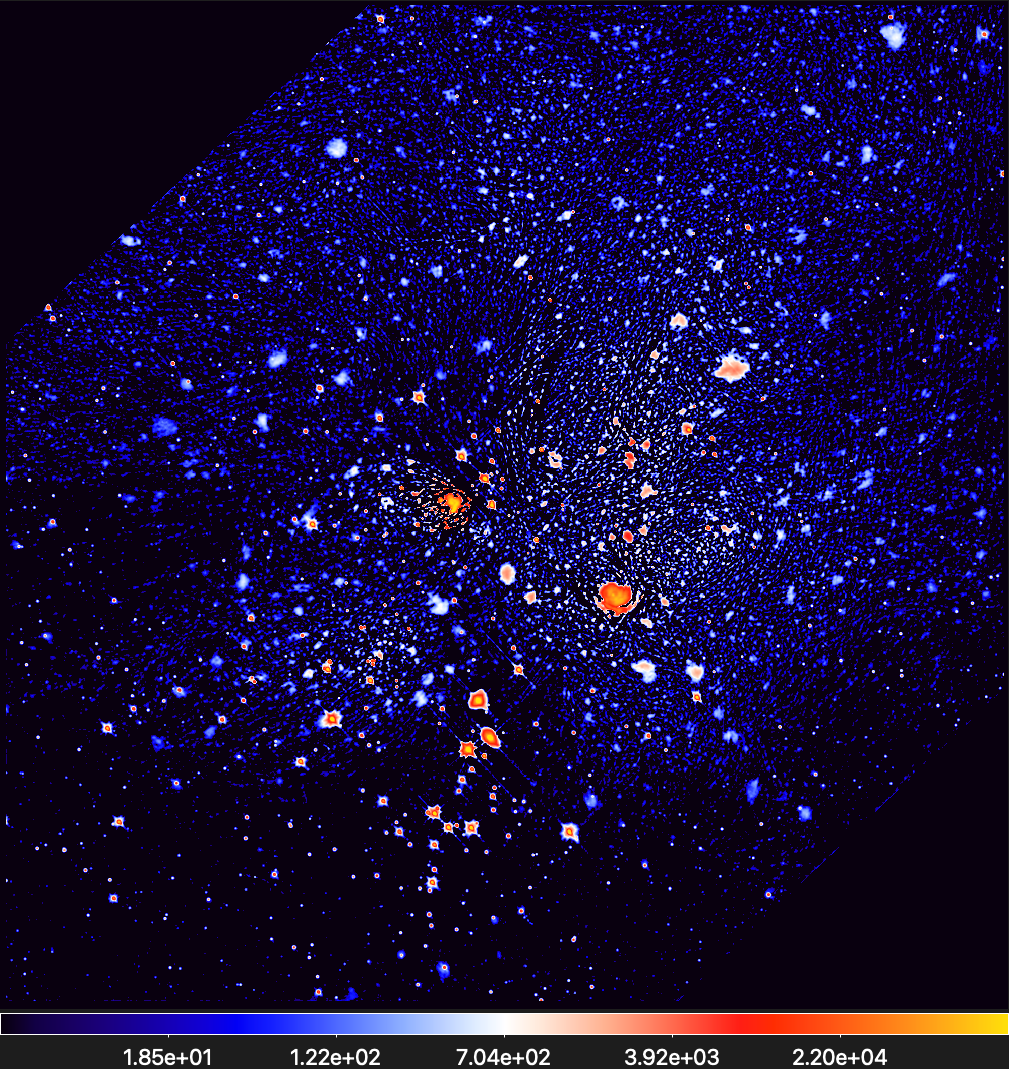
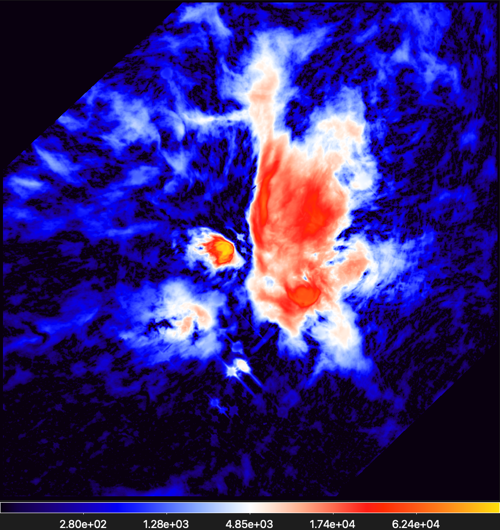
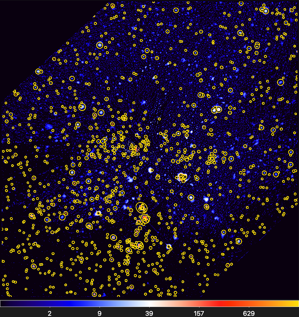
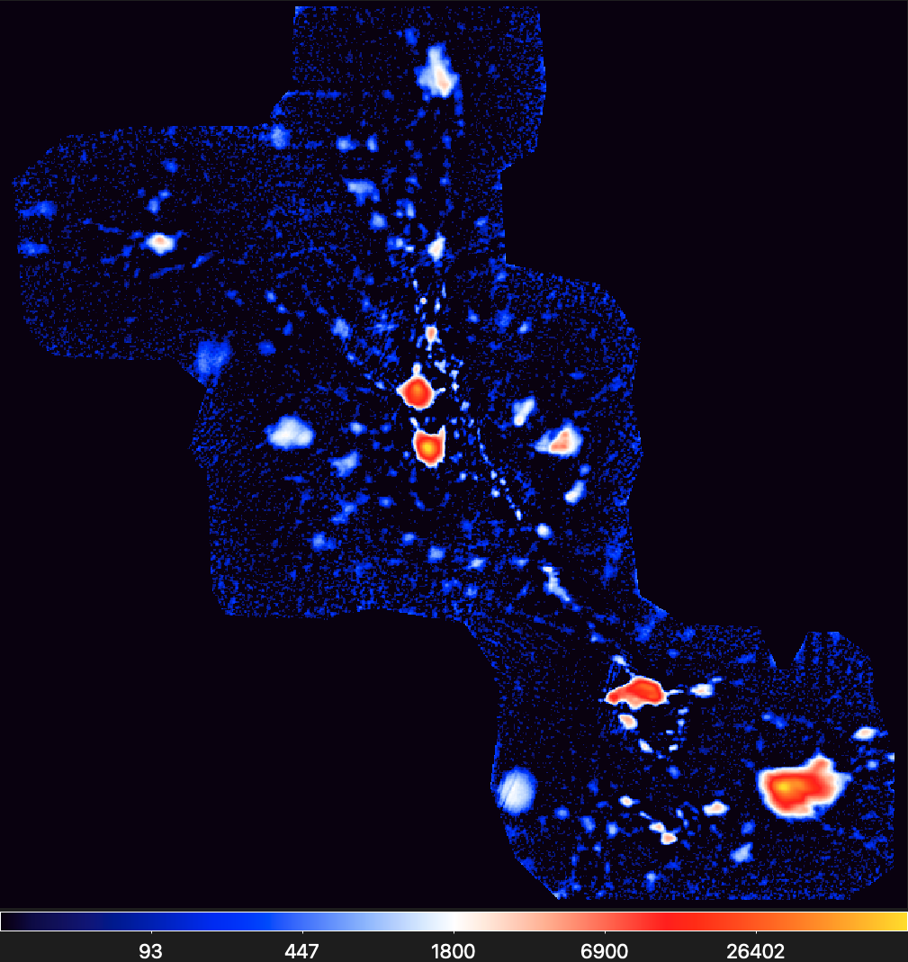
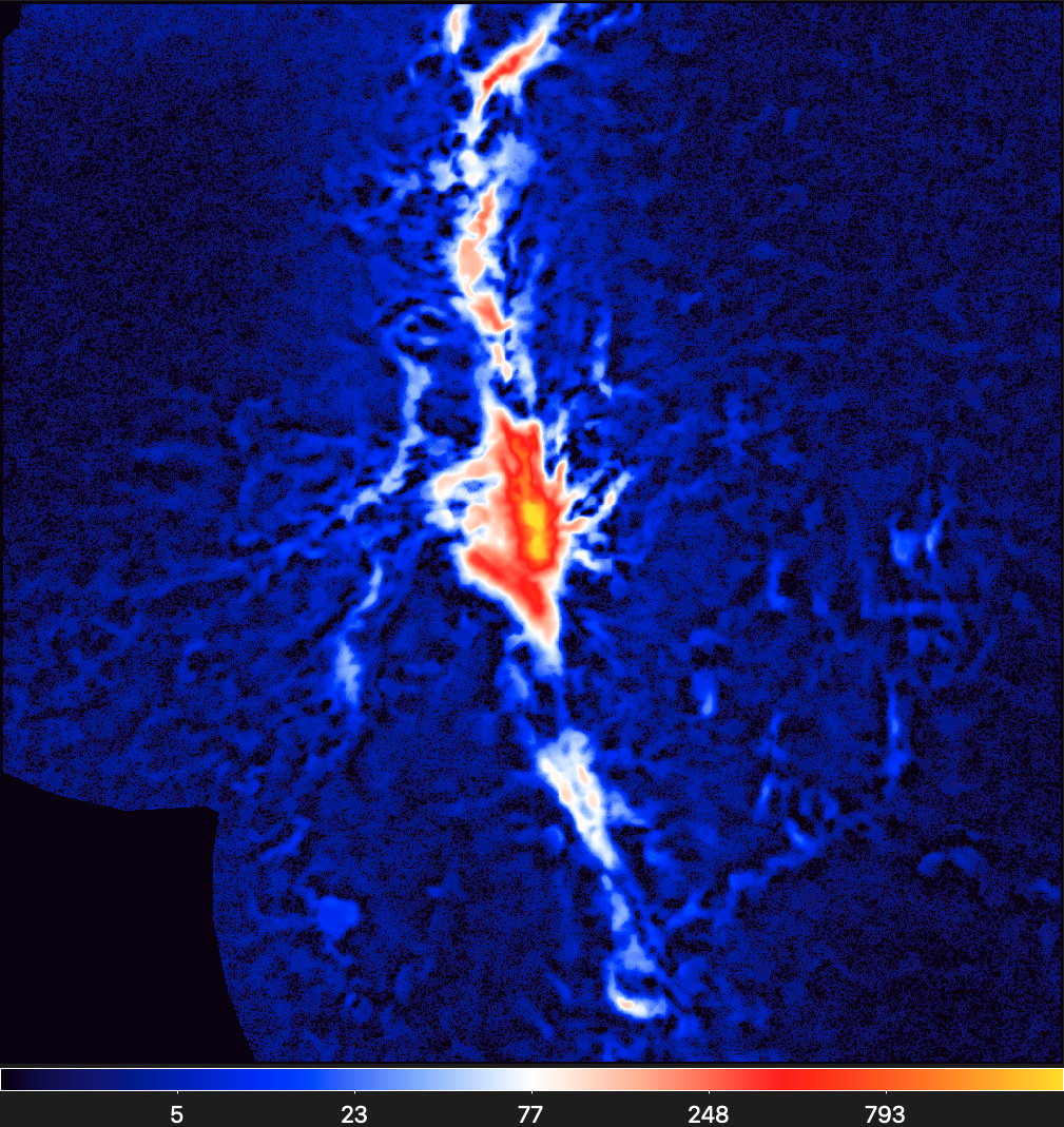
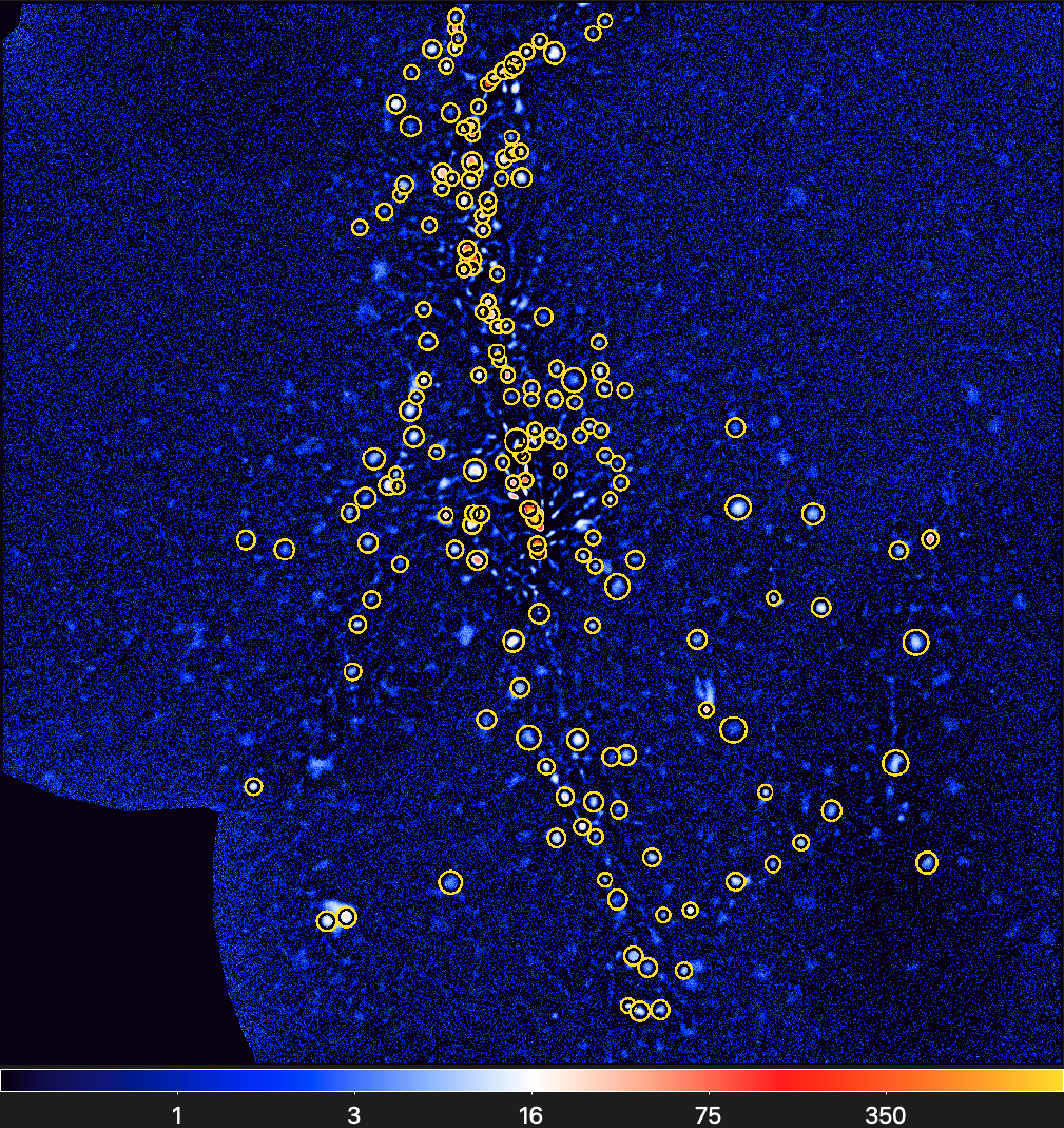
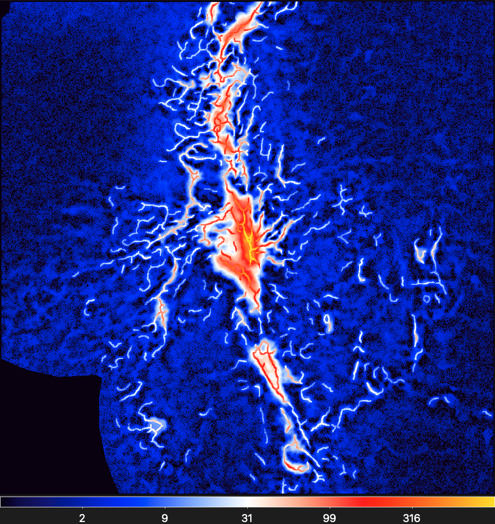
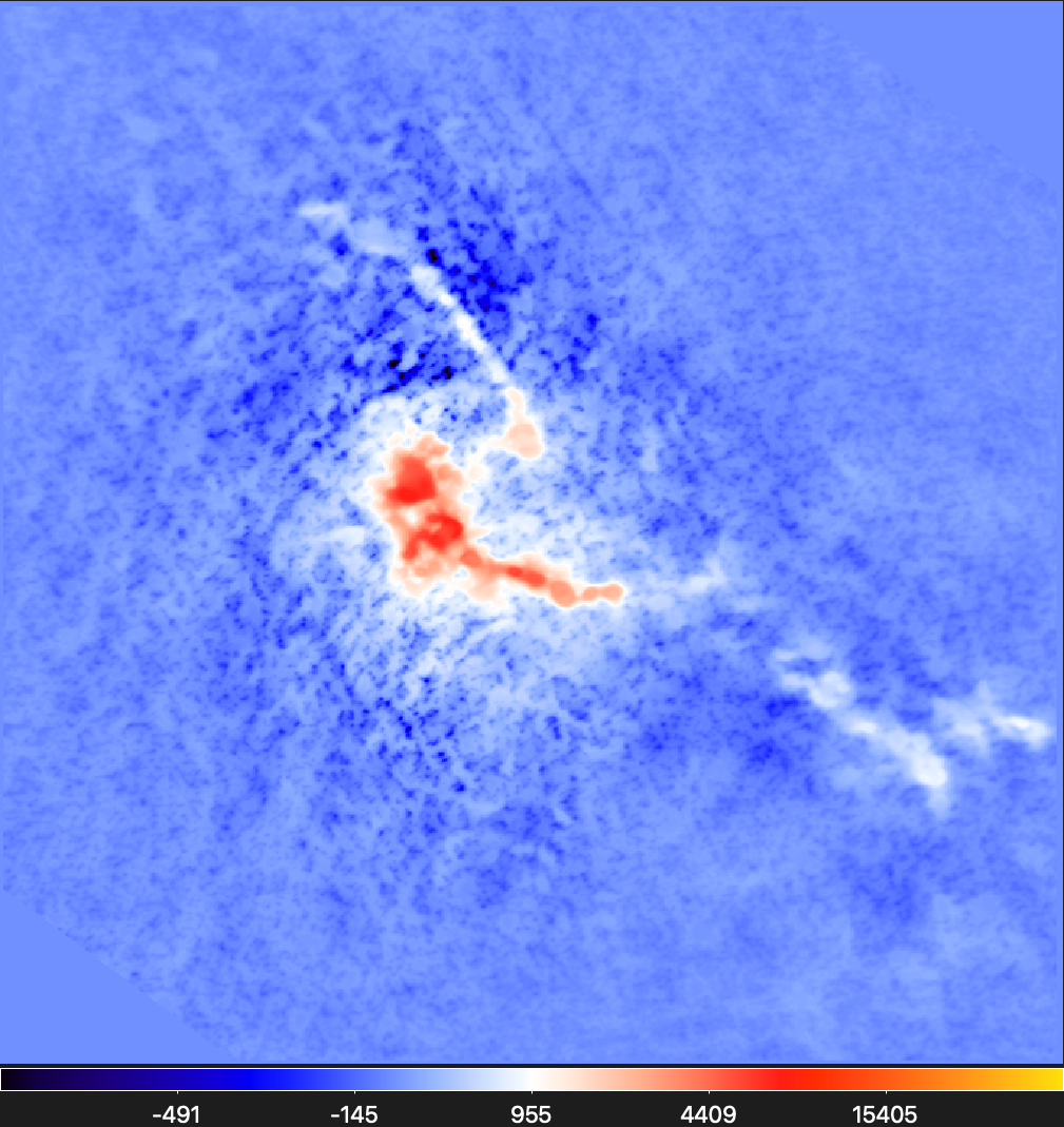
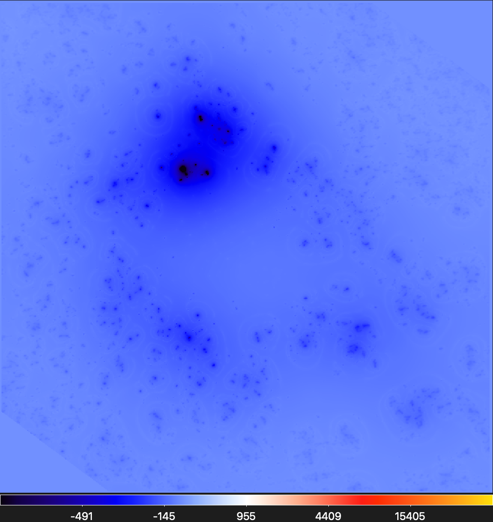
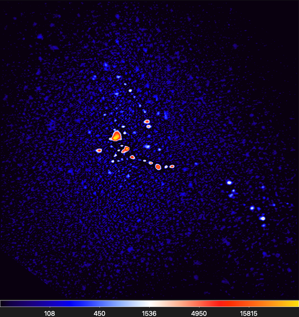
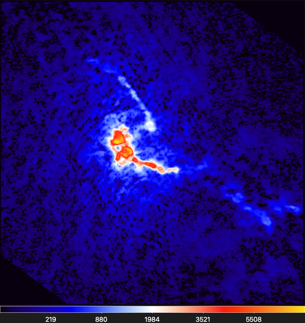
Star-Forming Cloud L1688
L1688 was observed with Spitzer in the IRAC 8 μm waveband
(Evans et al 2009). The
image below with an angular resolution of
6" shows a complex intensity distribution in this well-known star-forming region, with the
background varying by almost two orders of magnitude and many sources situated in both faint and bright background areas. For this
source and filament extraction with getsf, a maximum size of
30" of the sources and filaments of interest was adopted.
Spitzer (IRAC) image at 8 microns

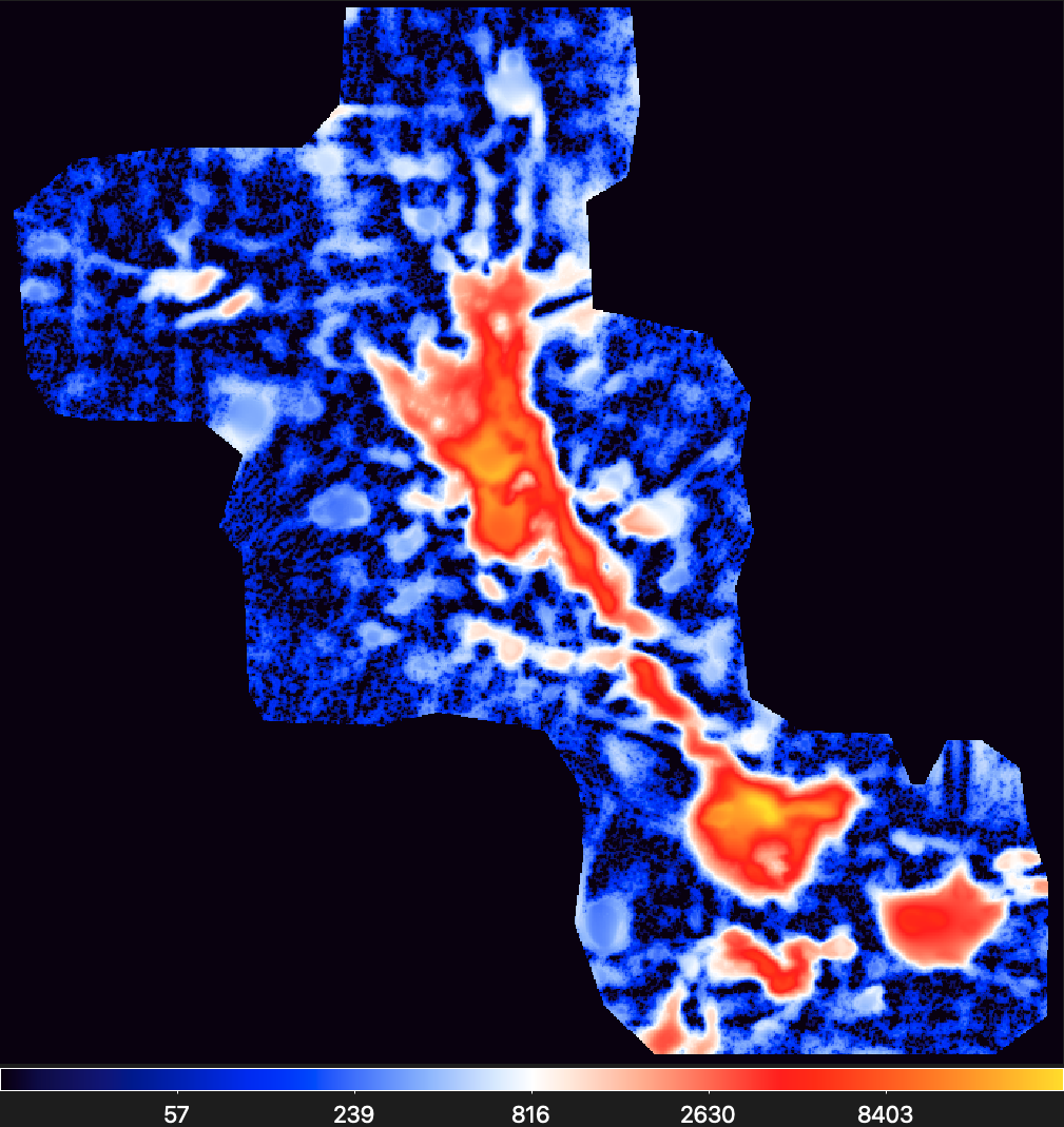
Background of sources
Background of filaments
Component of sources
Component of filaments
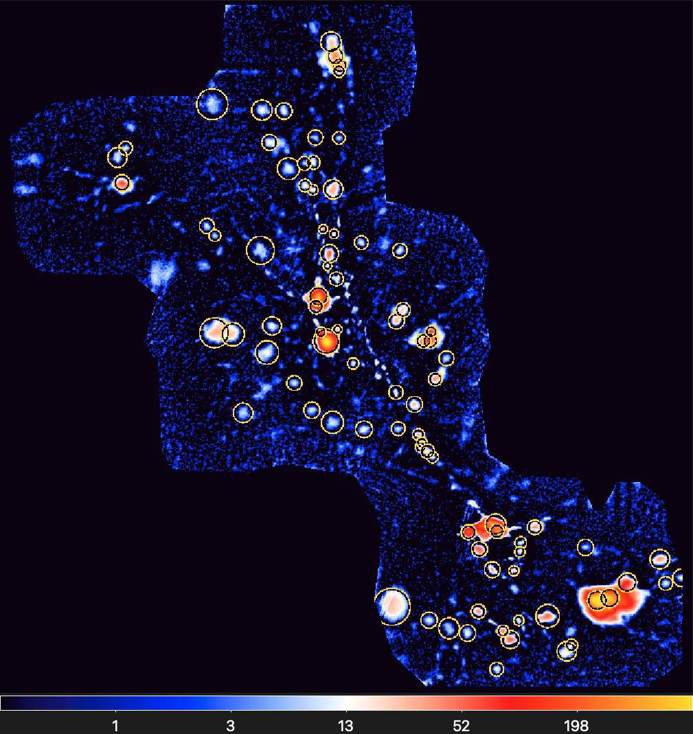
Extracted sources (footprints)
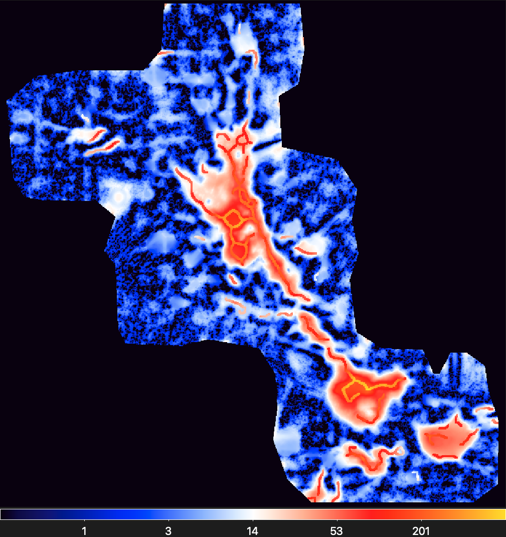
Extracted filaments (skeletons on scales 6–30")
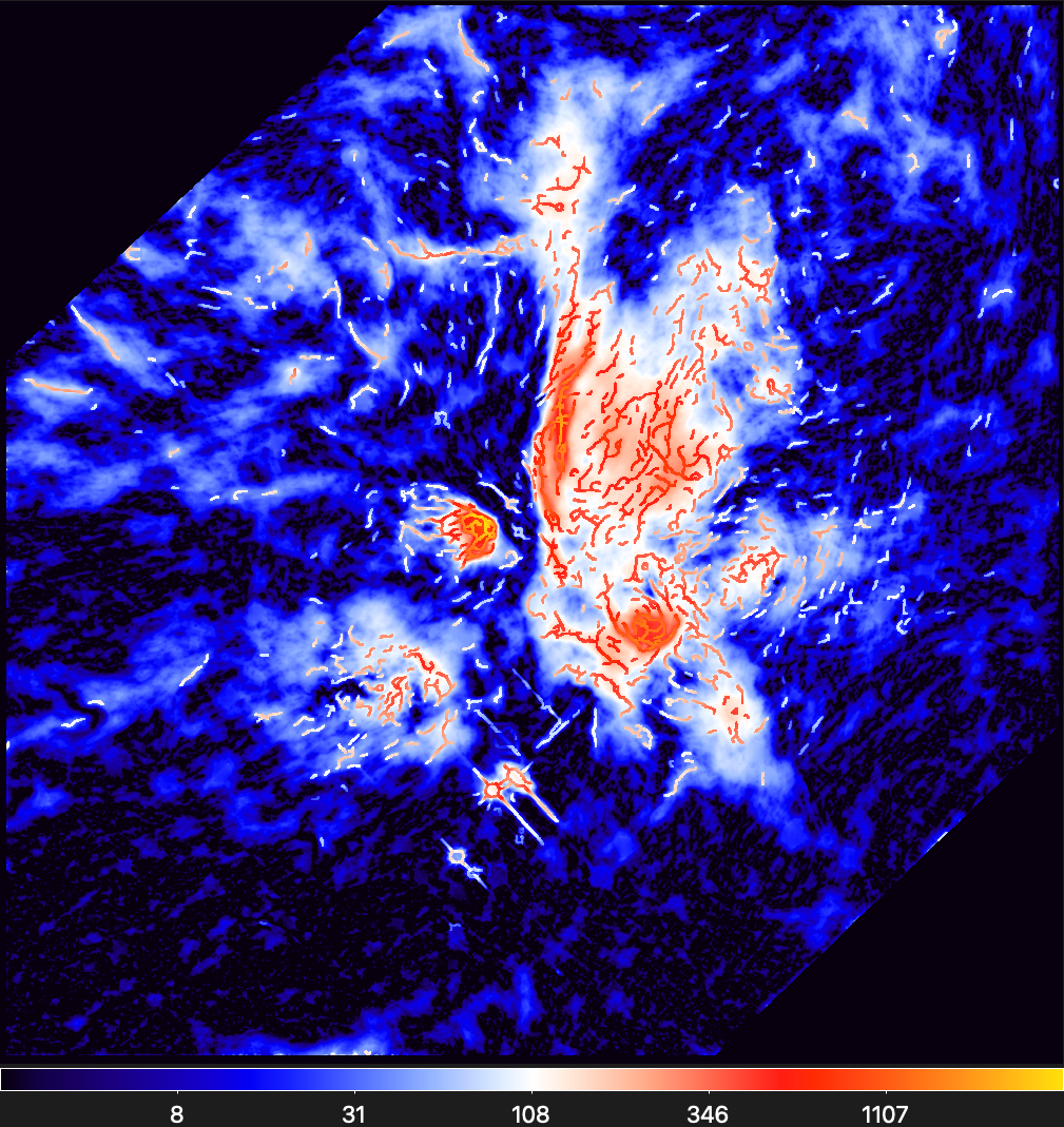
Extracted filaments (skeletons on scales ~30")
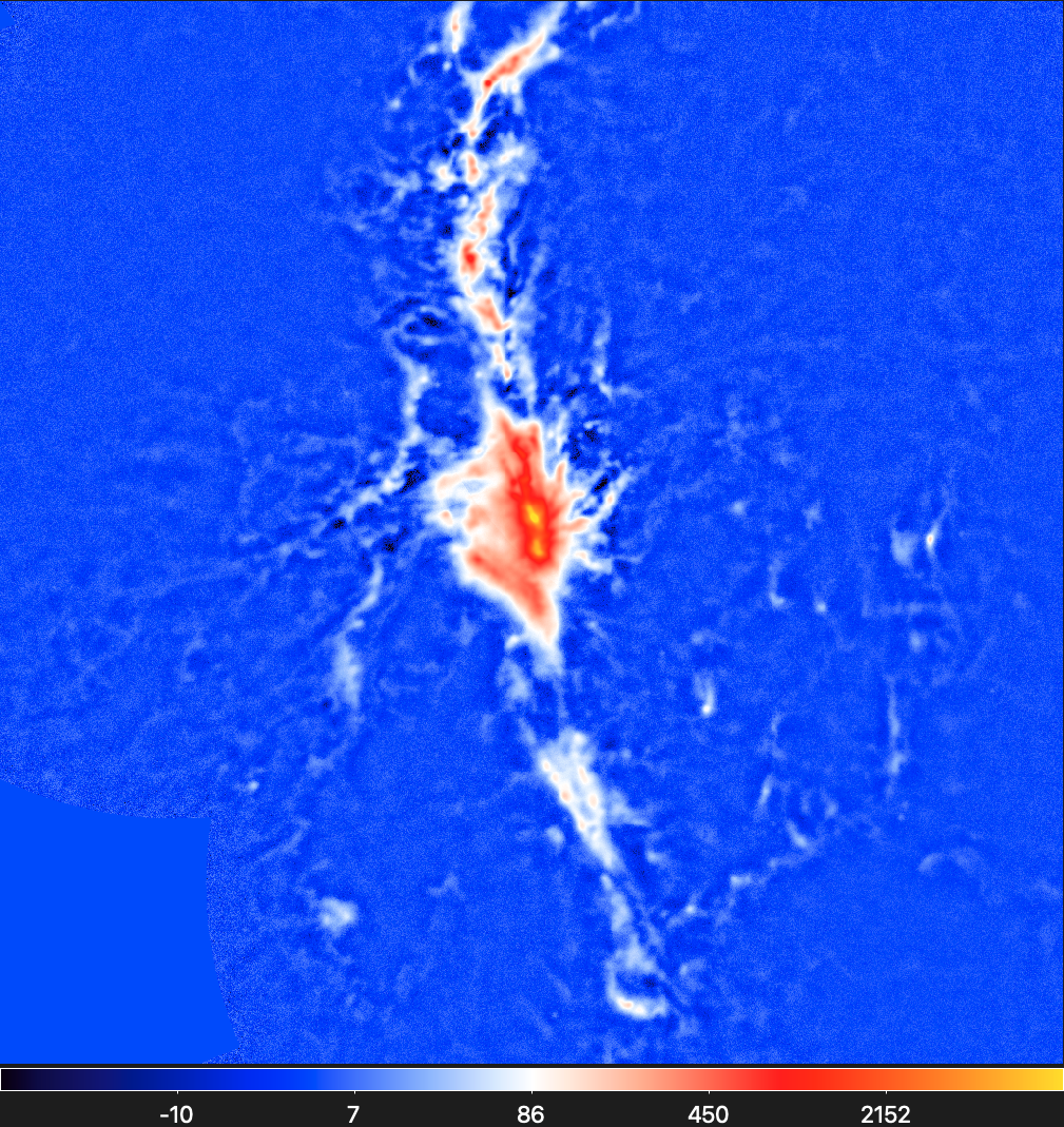
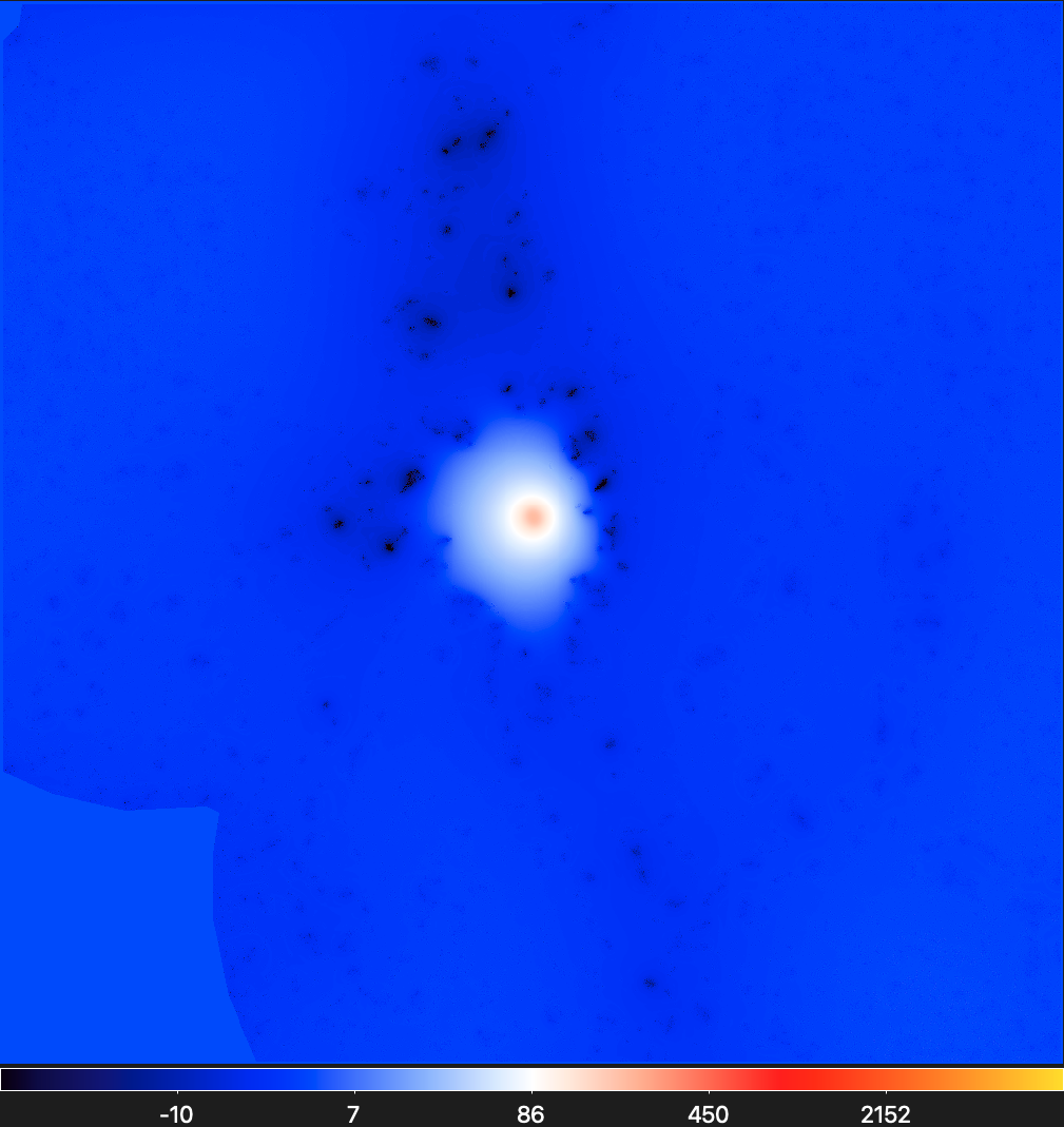
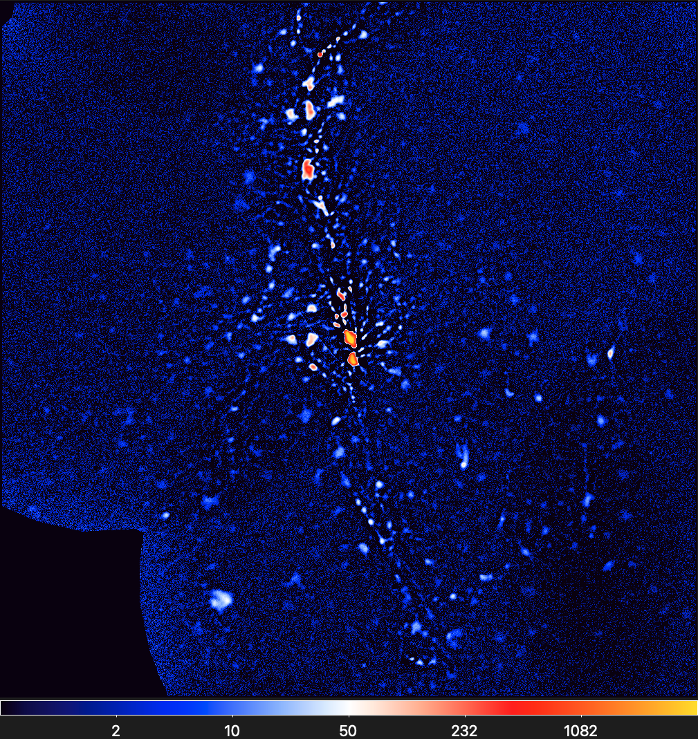
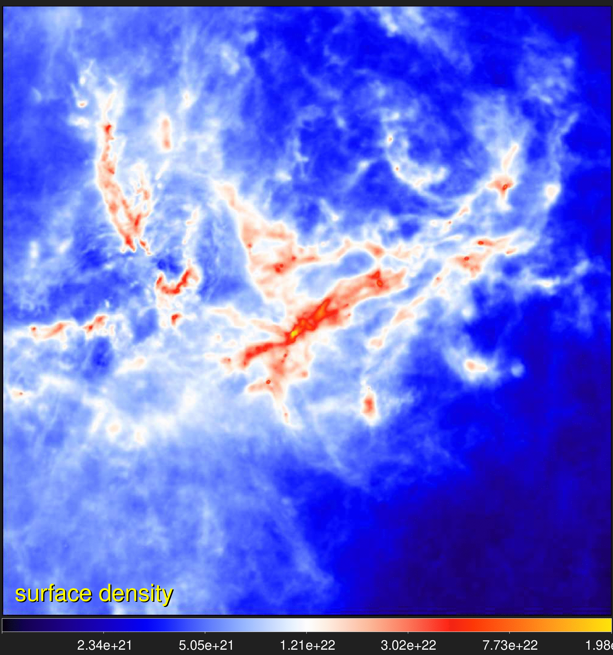
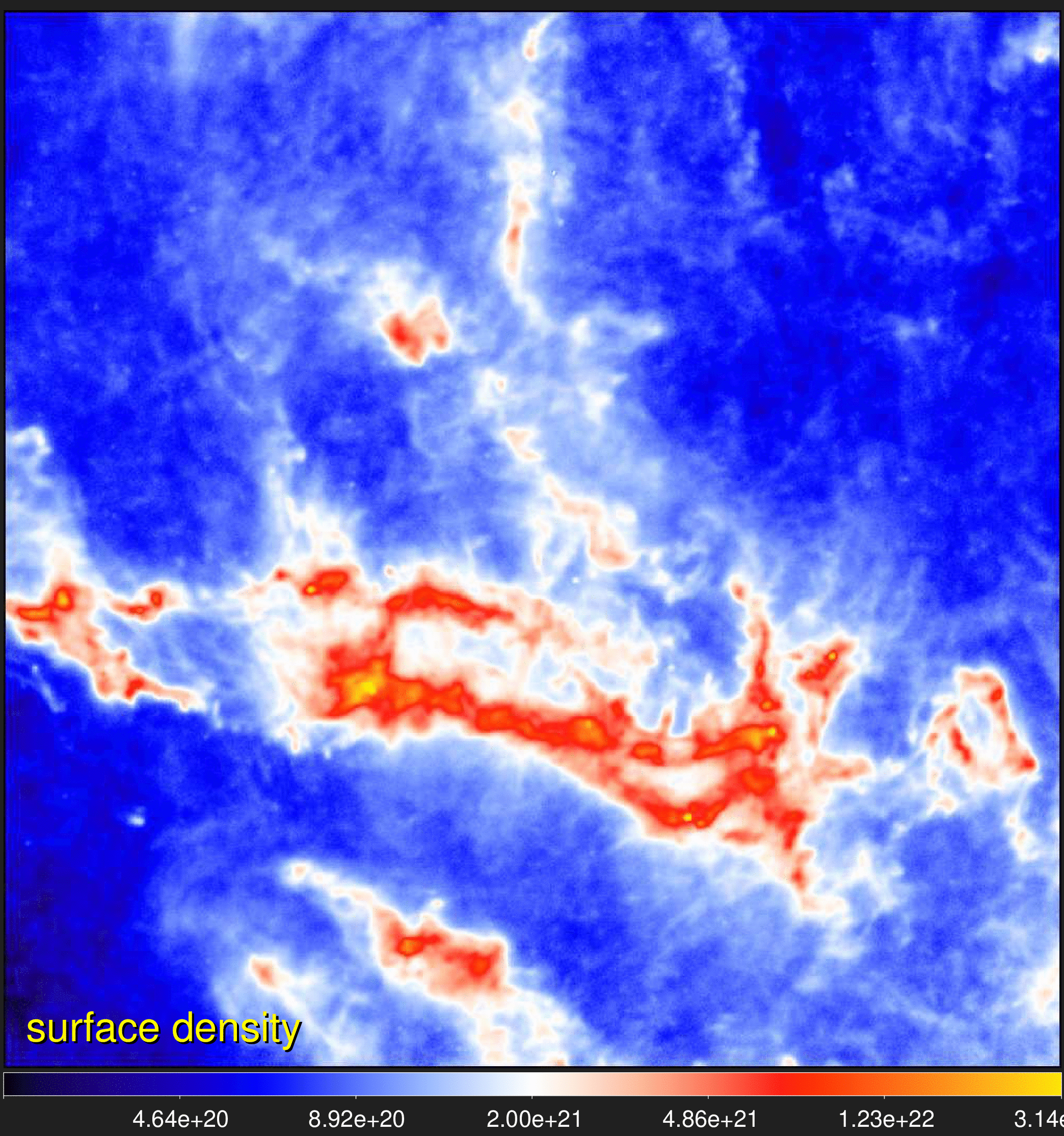
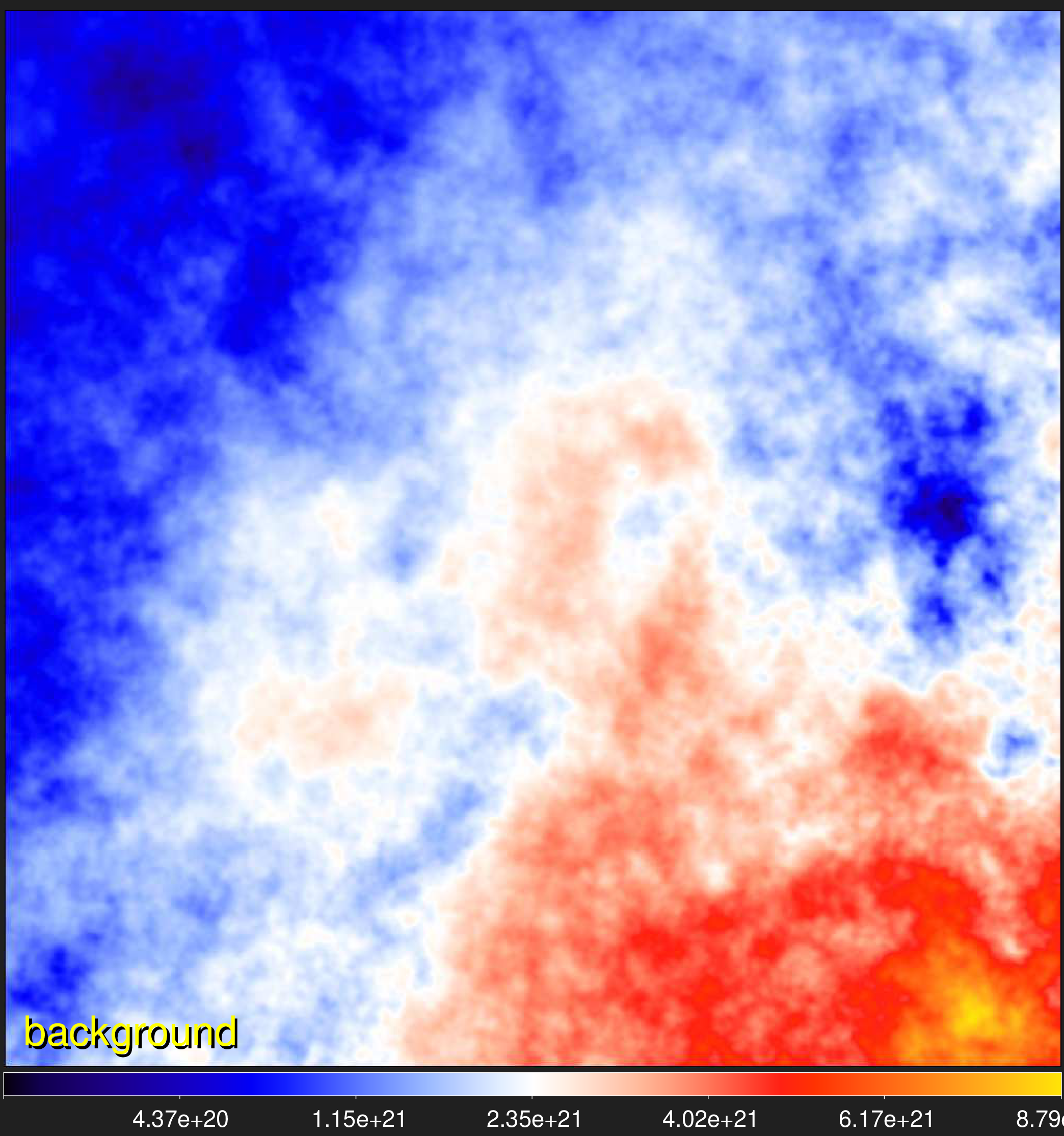
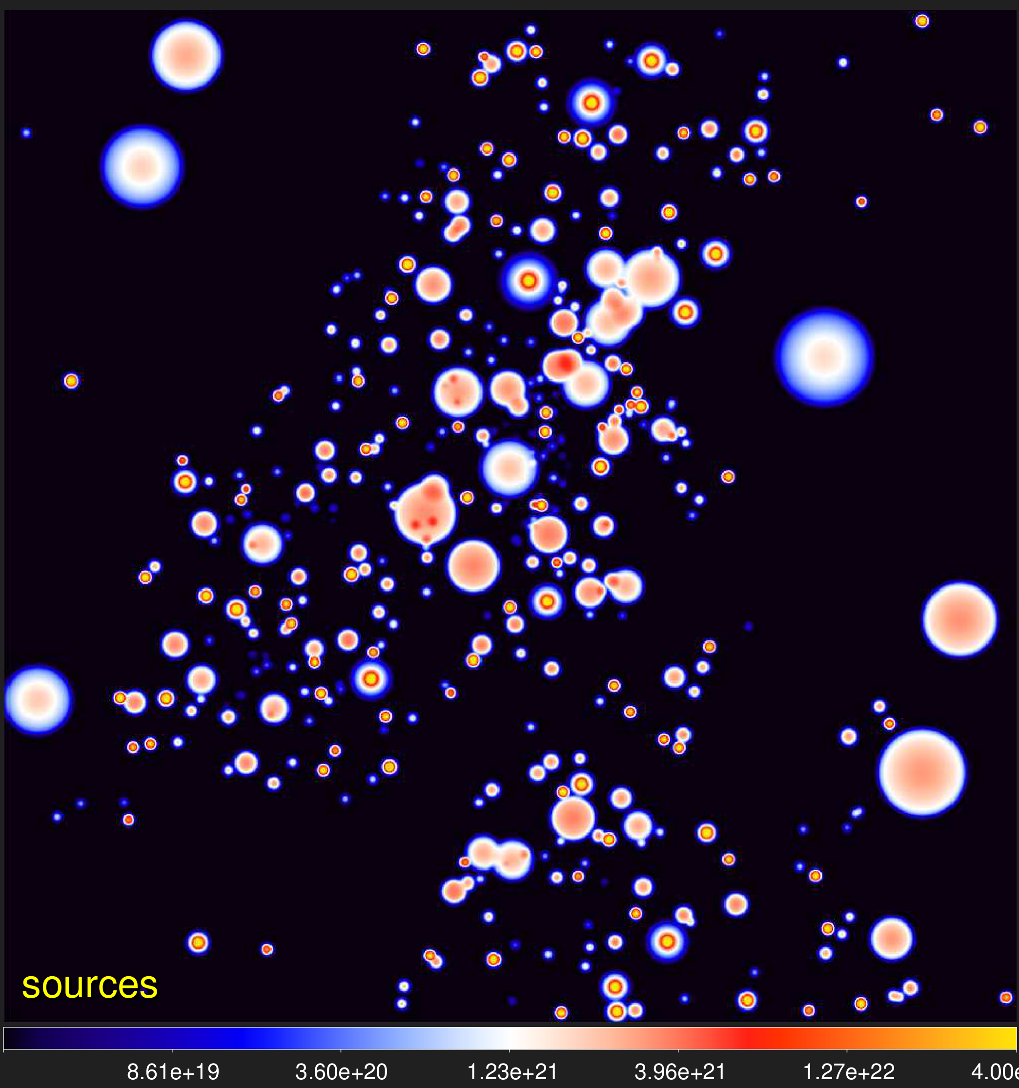
Embedded Starless Core L1689B
L1689B, one of the nearest well-resolved starless cores (a distance of 140 pc) embedded in a resolved filament, was observed with
Herschel in five PACS and SPIRE wavebands (Ladjelate et al. 2020).
The 160–500 μm
images
were used to compute a high-resolution (13.5") surface density image to illustrate the
new extraction method on a single image. Besides the reduction of the number of images, the use of surface densities allows
getsf to catalog physical parameters of the core and filament.
For this source and filament extraction with getsf, a maximum size of
90" of the sources and 180" of the filaments of interest
was adopted.
High-res (13.5") surface density
Background of sources
Background of filaments
Component of sources
Component of filaments
Extracted sources (footprints)
Extracted filaments (skeletons on scales 14–200")
Extracted filaments (skeletons on scales ~200")
Star-Forming Cloud NGC6334
NGC6334 was observed with APEX at 350 μm, equipped with the ArTéMiS camera
(André et al. 2016). The
image below
with an angular resolution of 8" represents an improvement by a factor of 3 with respect to
the Herschel images at 350 μm. Subtraction of the correlated sky noise resulted in
the image that has no signals on spatial scales above 120"
(André et al. 2016). Therefore,
the large-scale background and the zero level of the image are not known and the structures in the image are smaller than the largest
scale. Fortunately, such observational problems are totally unimportant for getsf.
For this source and filament extraction with getsf, a maximum size of
30" of the sources and filaments of interest was adopted.
APEX (ARTEMIS) image at 350 microns
Background of sources
Background of filaments
Component of sources
Component of filaments
Extracted sources (footprints)
Extracted filaments (skeletons on scales 8–30")
Extracted filaments (skeletons on scales ~30")
Star-Forming Cloud Orion A
Orion A was observed with JCMT at 450 and 850 μm
with the SCUBA-2 camera (Lane et al. 2016) with angular resolutions of
9.8" and 14.6", respectively. The
850 μm
image below displays the northern
part of the integral-shaped filament (ISF). Like with other ground-based submillimeter observations that must subtract sky background,
large-scale emission in the images has been filtered out (Kirk et al. 2018).
For this two-wavelength getsf extraction in both 450
and 850 μm images, a maximum size of {20, 30}" of the sources
and {30, 45}" of the filaments of interest was adopted.
JCMT (SCUBA-2) image at 850 microns
Background of sources (850 microns)

Background of filaments (850 microns)
Component of sources (850 microns)
Component of filaments (850 microns)
Extracted sources (footprints)
Extracted filaments (skeletons on scales 14.5–45")
Extracted filaments (skeletons on scales ~45")

Star-Forming Cloud W43-MM1
W43-MM1 was observed with the 12-m array of the ALMA interferometer (baselines 13–1045 m) in the 233 GHz band centered
at 1300 μm (Motte et al. 2018;
Nony et al. 2020). The small image below with an angular resolution of
0.44" contains spatial scales of up to 12", beyond which
the interferometer was insensitive to the emission. For this source and filament extraction with
getsf, a maximum size of 0.8" of the sources
and 1.3" of the filaments of interest was adopted.
ALMA (12-m array) image at 1.3 mm
Background of sources
Background of filaments
Component of sources
Component of filaments
Extracted sources (footprints)
Extracted filaments (skeletons on scales 0.8–1.3")

Extracted filaments (skeletons on scales ~2")
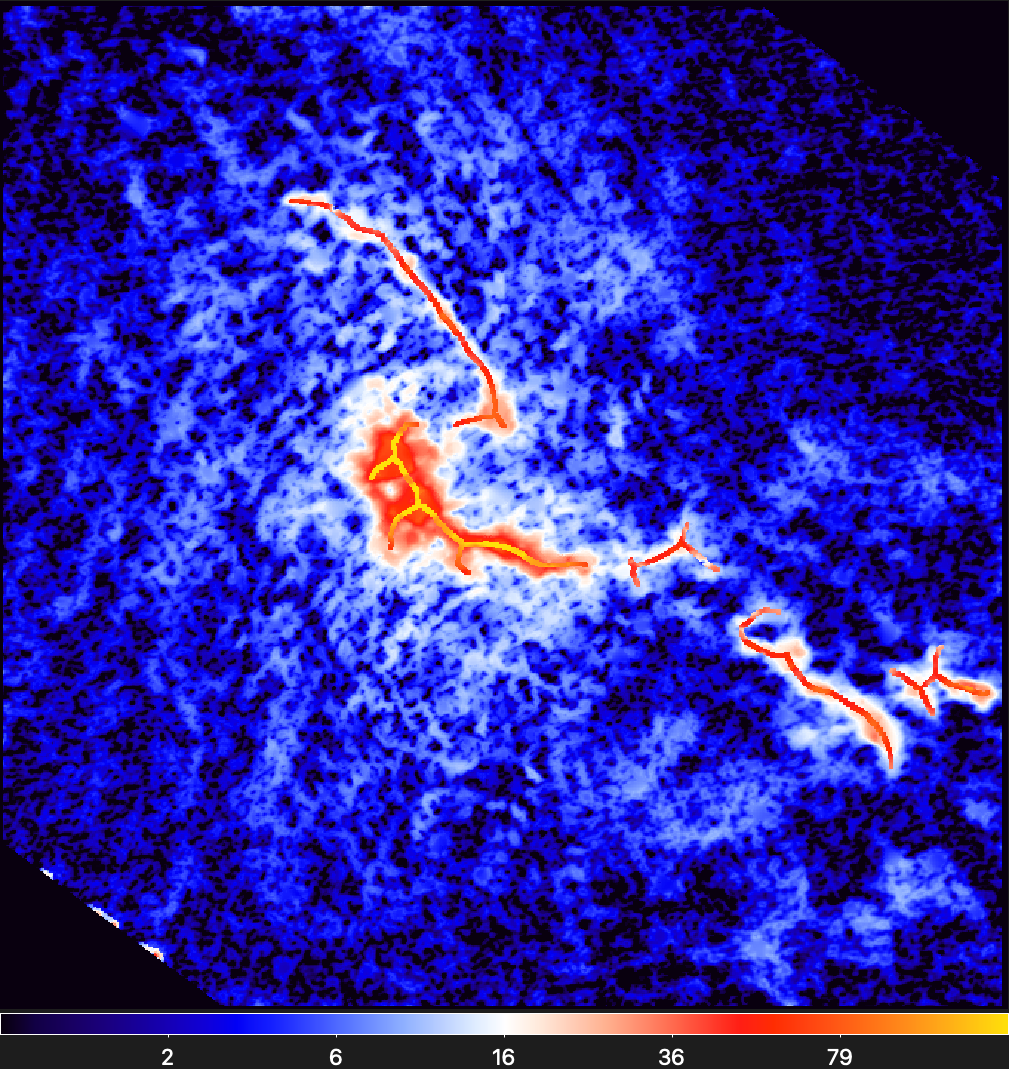
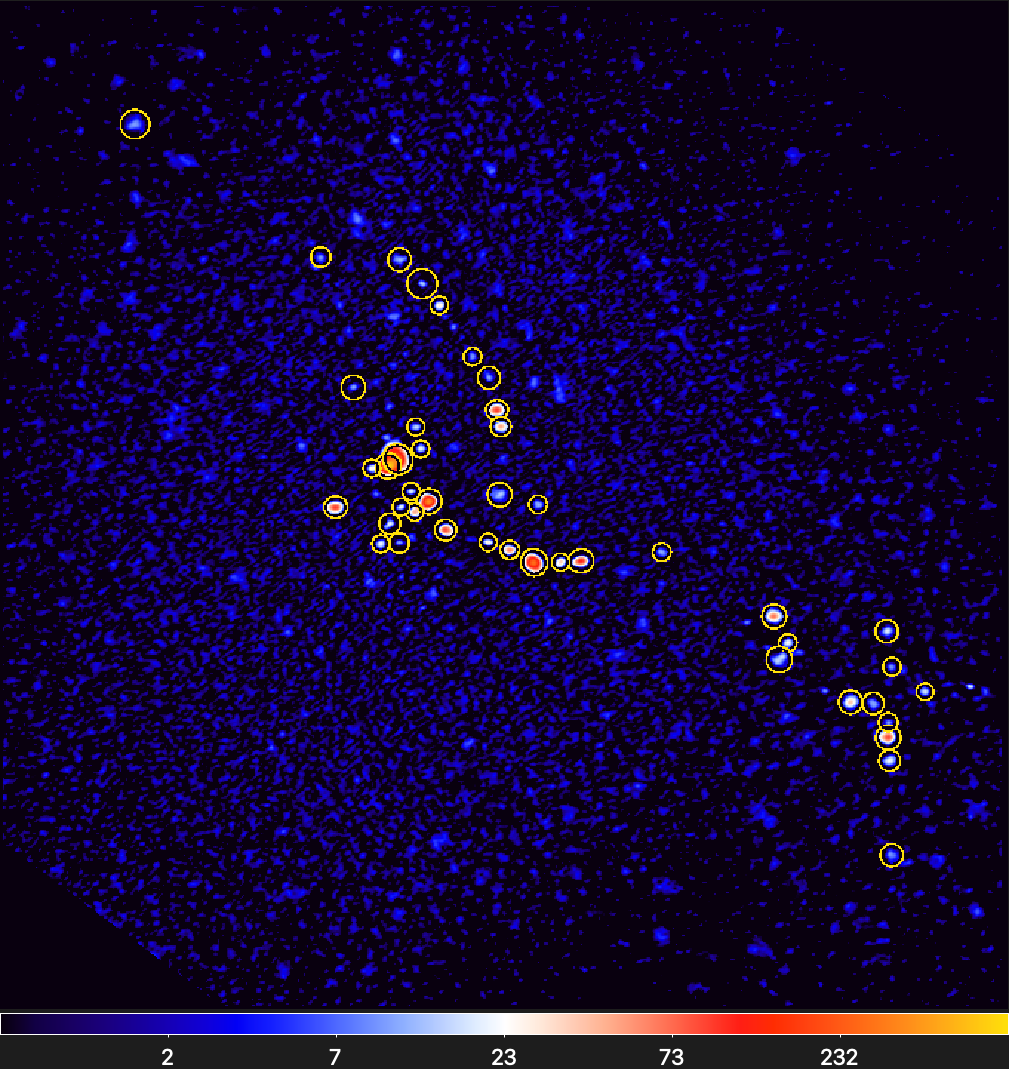
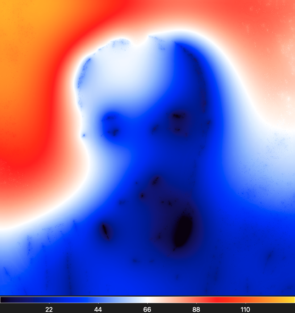
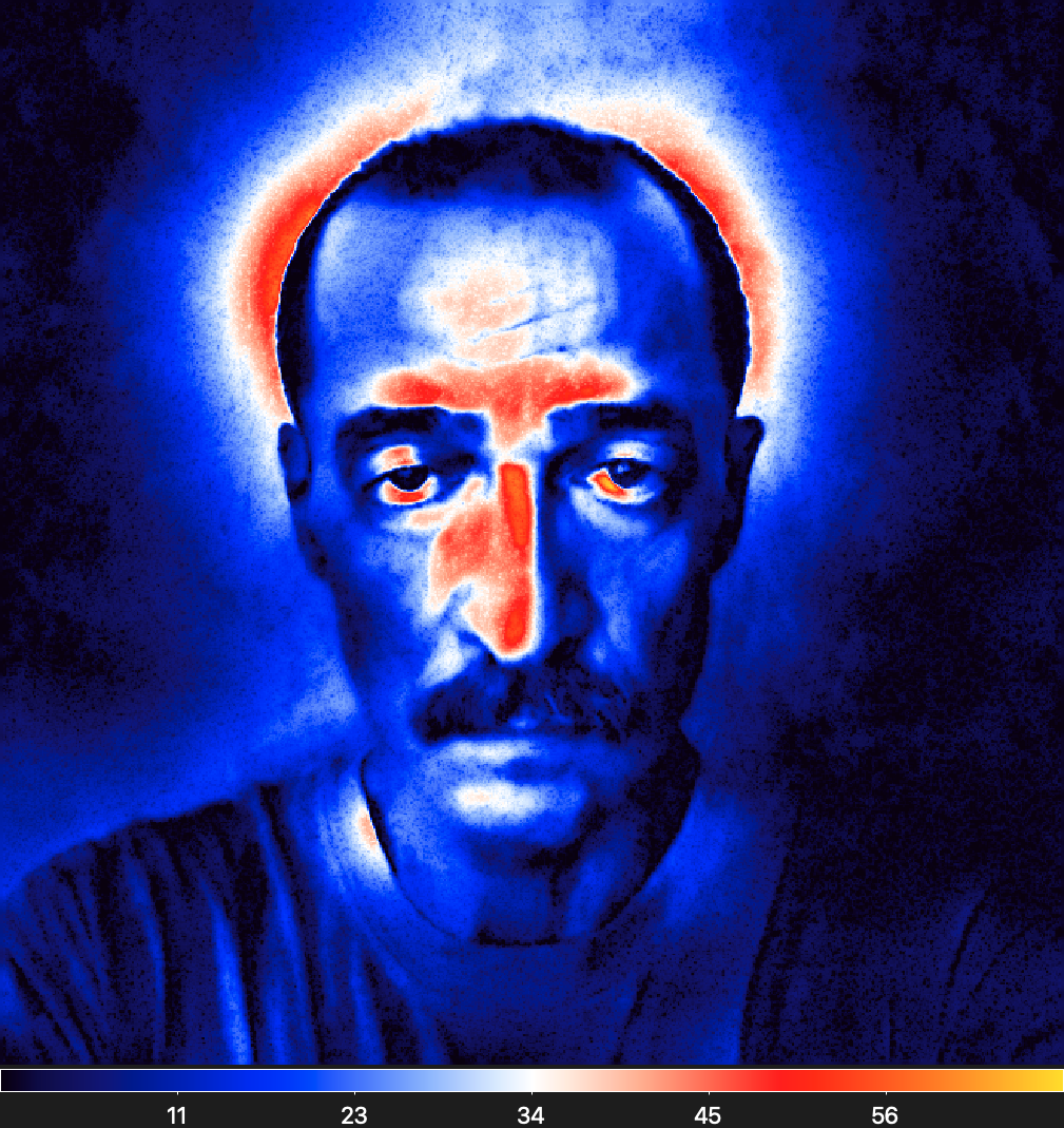
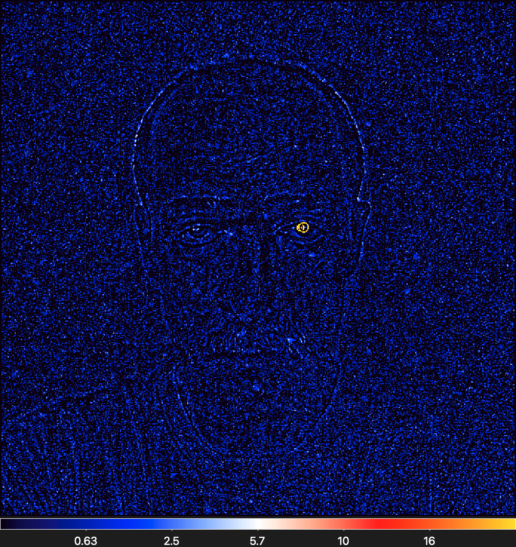
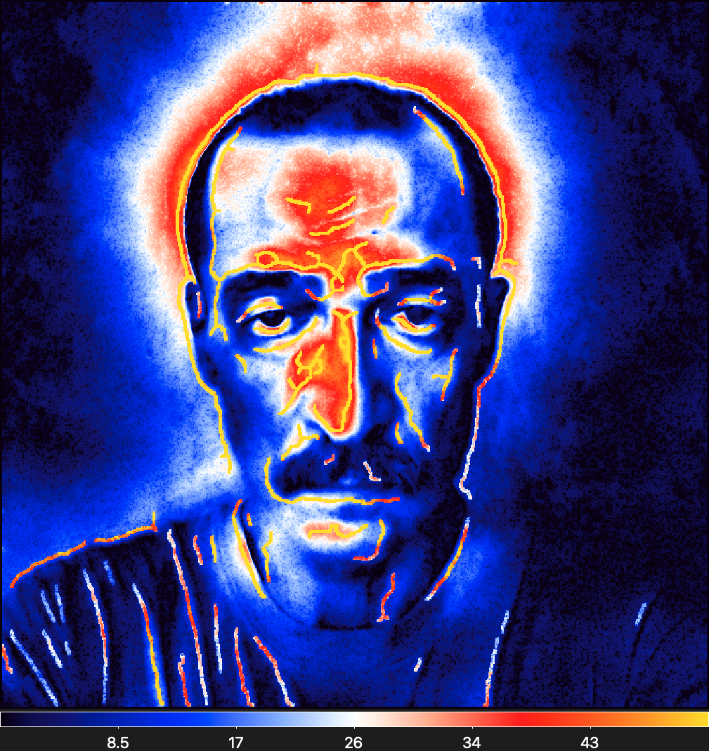
Sasha
This man photographed himself in July 2019 with a smartphone Samsung Galaxy S9 Edge from a distance of ~60 cm.
The JPEG image was then converted to the FITS format using ImageMagick
and the resulting 661 × 661-pixels image was arbitrarily assigned a 2" pixel size
and an angular resolution of 6". The pixel values were assumed to have the units of MJy/sr.
For this source and filament extraction with getsf, a maximum size of
6" of the sources and 15" of the filaments of
interest was adopted.
Original Image
Background of sources
Background of filaments
Component of sources

Component of filaments
Extracted sources (footprints)
Extracted filaments (skeletons on scales 6–15")
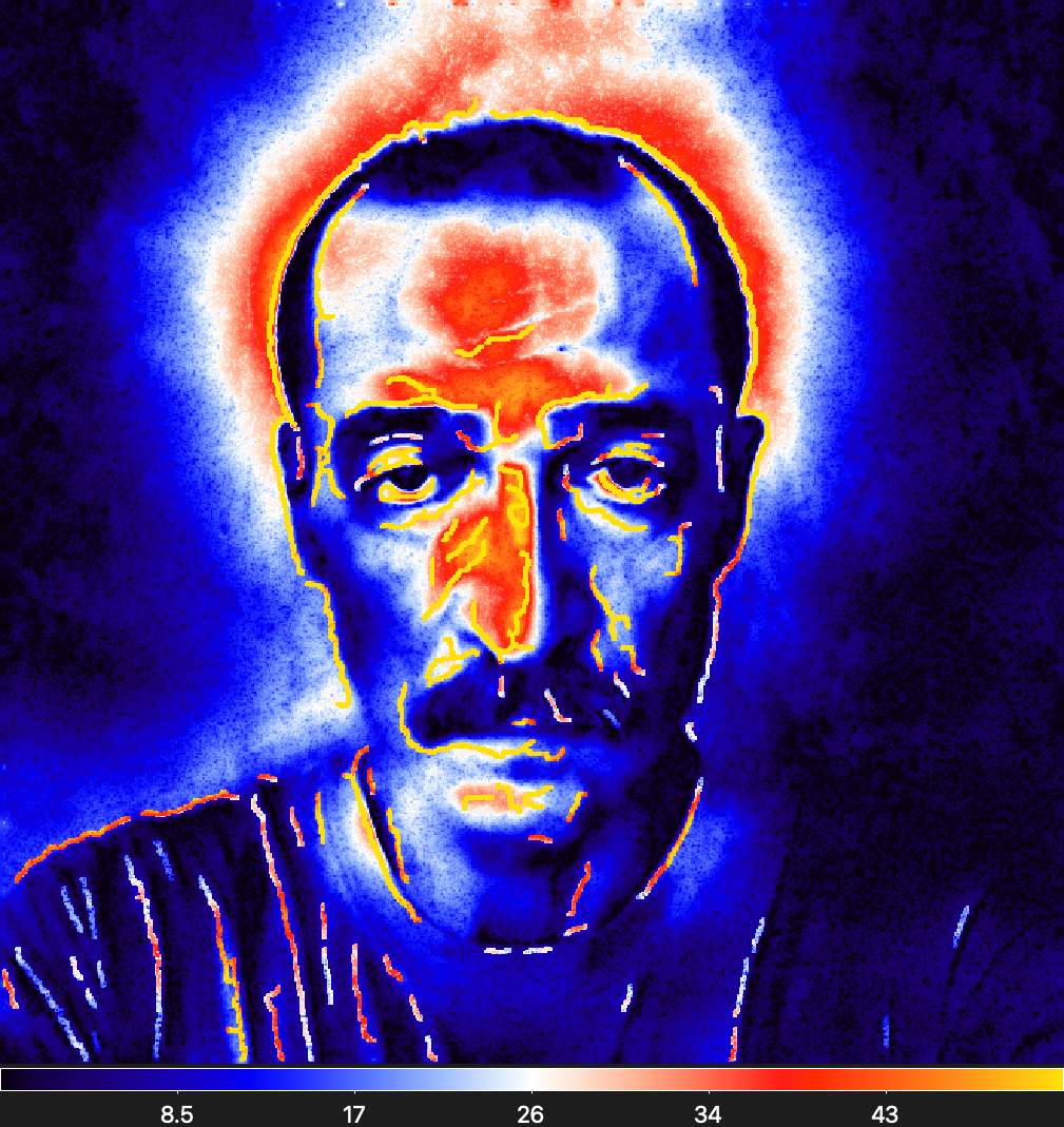
Extracted filaments (skeletons on scales ~15")
< Support
Method >
")
Extraction Method
Flexible multi-wavelength design enables getsf to handle from one up to 99 images,
not necessarily all of them observed in different wavebands. Any subset of the input images, deemed beneficial for the detection
purposes, can be used to identify the sources and filaments, whereas measurements of the detected sources and filaments are
provided for all input images. In a non-standard application, the method can also be employed for the position-velocity cubes,
if the latter are split into separate images along the velocity axis. The method is almost universally applicable – it
has been tested on a very wide range of various astronomical observations, numerical simulations, and even digital photographs.
The method is designed and expected to work for all "normal" images, that are not very sparse: most pixels must contain detectable
signals (measurable data). Examples of the images, for which getsf might not produce
reliable results, are some extremely faint X-ray or UV low-count images that have isolated spiking pixels, surrounded by
large areas of pixels that were not assigned any detectable signal. On the other extreme, the images suitable for
getsf must not be extremely smooth: they must have some variations on spatial
scales of the order of angular resolution. For both types of non-standard images, getsf
would still work and complete extractions, but its results might not be reliable. This is because the method relies on the standard
deviations of the background or noise fluctuations outside structures at each of its processing steps and the values in such unusual
images may not correctly represent the statistics of the observed data.
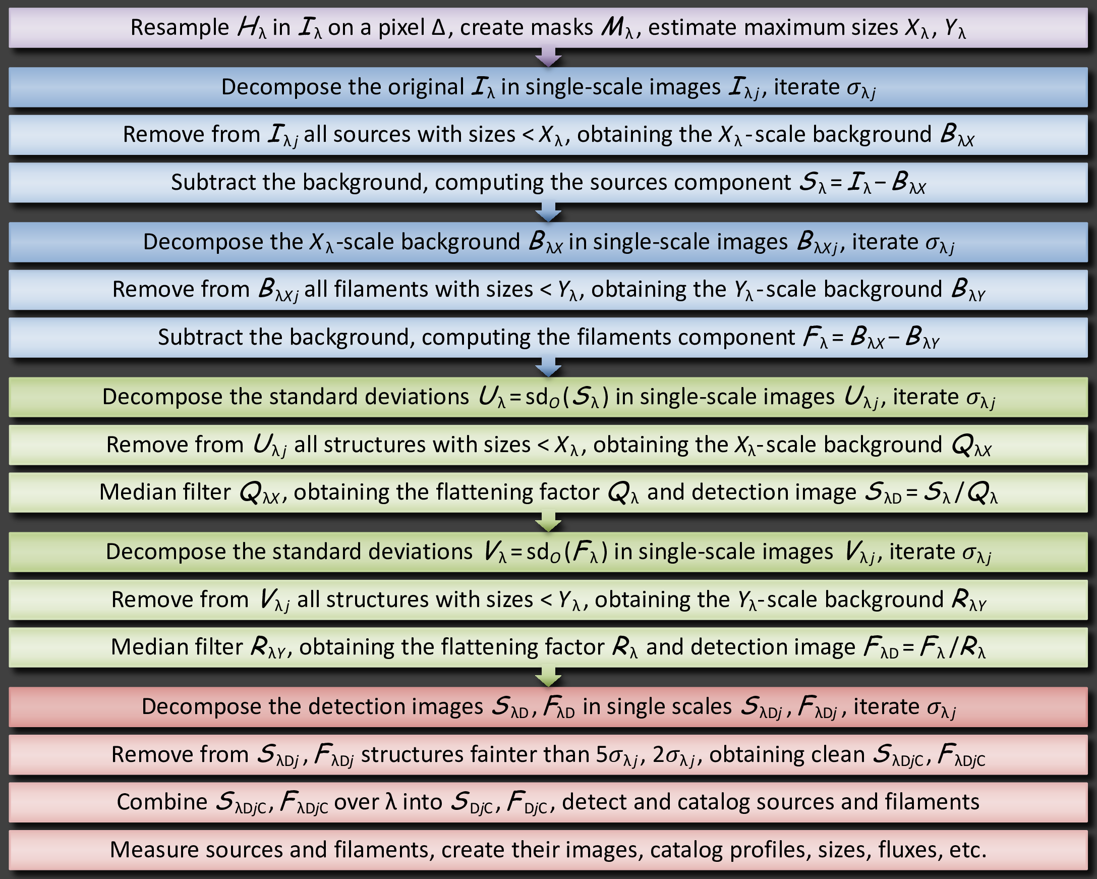
Main processing steps of getsf:
-
Preparation of a complete set of images on the same grid of pixels and optional derivation of high-resolution surface densities
and dust temperatures.
-
Separation of the structural components of sources and filaments from each other and from their backgrounds using spatially
decomposed images.
-
Flattening of the residual noise and background fluctuations in the images of the separated components of sources and filaments.
-
Combination of the flattened components of sources and filaments over several (or all) wavebands in their spatially decomposed
images.
-
Detection of sources (positions) and filaments (skeletons) in the combined images of the components in their spatially decomposed
images.
-
Measurements of the properties of detected sources and filaments, creation of the multi-wavelength output catalogs and images.
In the getsf flowchart, the colored blocks highlight the steps of
preparation, background subtraction,
image flattening, and extraction of sources and filaments:
The method has a single user-definable parameter (per image): the maximum size of the structures of interest to extract.
This parameter is determined by users from the images on the basis of their research interests.
Before starting any extraction, it is necessary to formulate the aim of the study – what structures of interest must be
extracted. The method knows and is able to separate three types of structures: sources, filaments, and backgrounds. To separate
the structural components with getsf, the maximum size
X of the sources and Y of the filaments
of interest need to be manually (visually) estimated from the prepared images, independently for each waveband. This can be
accomplished by opening an image in ds9, finding the largest structure
of interest, and placing a circular region, fully covering its width.
The maximum sizes X and Y are defined as the
footprint radii (arcsec) of the largest source and the widest filament, respectively, to be extracted. A footprint size has the meaning
of a full width at zero (background) level: the largest two-sided extent from a source peak or filament crest, where that structure is
still visible in the image against its background. For a Gaussian intensity distribution, the footprint radius is slightly larger than
the half-maximum width H. For a power-law intensity profile, the footprint radius may become
much larger than H. If the widest filaments of interest are blended (overlapping each other
with their footprints), the Y values must be increased accordingly, to approximate the full
extent of the blend. In contrast, it is not necessary to adjust X for blended sources,
because their final backgrounds are determined from their footprints at the measurement step.
It is not necessary (also not possible) to evaluate the maximum size parameter X and
Y very precisely, a 50% accuracy is quite sufficient. Its purpose is to set a reasonable
limit to the spatial scales, when separating the structural components, and to the size of the structures to be measured and cataloged.
Indeed, getsf works with spatially-decomposed images and it needs to know the maximum
scale. It makes no sense to perform the decomposition up to a very large scale, if the extraction is aimed at much smaller sources or
narrower filaments. The method has no limitations with respect to the sizes (widths) of the structures to extract. However, it is
important to avoid detecting, measuring, and cataloging the peaks that are unnecessarily too wide, because they would likely overlap
with other sources of interest, which potentially would make their measurements less accurate.
Preparation of images
High-resolution surface density

Separation of components
Spatial decomposition (4–1400",
selected scales)
Component of sources
Background of sources
Component of filaments
Background of filaments
Taurus, Aquila, and IC 5146
The surface densities of the filaments in three well-studied star-forming regions in Taurus, Aquila, and IC 5146 were derived
from their images (at 160–500 μm) obtained with the
Herschel Space Observatory (HGBS key project, Ph. André).
They demonstrate that the observed filaments are highly sub-structured and their shapes, traced by their skeletons, are very
different on various spatial scales. Therefore, when studying filaments, it is necessary to detect their skeletons on those scales
that correspond to the widths of the structures being studied.
Taurus filaments on scales
18–576"
Aquila filaments on scales
18–576"
IC 5146 filaments on scales
18–576"
< Intro
Code >
")
Numerical Code
The method has been developed as a Bash script getsf that executes a suite of
utilities doing most of the numerical computations. Linux or macOS with
ifort
or gfortran can be used to install the code.
To read and write FITS images, it uses cfitsio
(Pence 1999); for resampling and reprojecting images,
it executes swarp
(Bertin et al. 2002); for determining source
coordinates (α, δ), it employs xy2sky from
wcstools
(Mink 2002); colored screen output is produced by
highlight (André Simon).
The latest version can be downloaded below. When downloading
getsf for the first time, users are requested to register to obtain
notifications on updated versions.
The initial reference version of the code and results of a
validation extraction can also be downloaded below. They are made available for
those who feel the need to have the same version of the code that was used in the published paper and for those who want to validate their
getsf installation and configuration file by comparing their results with a reference
extraction of sources and filaments in a very small simulated image.
Note that getsf may become corrected and/or improved in the future and that only the
most recent version is supported.
Notable Improvements or New Features
• Revision 220627 (new feature).
Starting with this version, getsf includes a new utility
makecube that allows creation of 3D data cubes from separate 2D images to facilitate
analysis of extraction results, primarily when running getsf on slices extracted from
line data cubes.
• Revision 220610 (new feature).
Starting with this version, getsf creates ds9
region files for both sources (half-maximum and footprint ellipses) and filaments (global and scale-dependent skeletons) to facilitate
their visualization and analyses. For best visibility of the shapes, getsf defines a set of
20 distinct colors:
gre
blu
ora
pur
cya
mag
lim
pin
tea
lav
bro
bei
mar
min
oli
apr
gra
red
yel
whi, in addition to hundreds of other colors recognized by the region files.
• Revision 210915 (new feature).
Starting with this version, getsf provides also the measurements of filaments for the
global skeletons the same way the measurements are done for the set of scale-dependent
skeletons.
• Revision 210907 (new feature).
Starting with this version, getsf adds the global,
scale-independent skeletons to its output. Several users experienced difficulties analyzing the complex nature of observed filaments with
the default set of scale-dependent skeletons produced by getsf. Responding to their needs,
the updated getsf produces also images of the global skeletons tracing the filamentary
structures on all scales, independently of the filament widths. They are created from the scale-dependent skeletons within the range of
scales of interest for the user, that is up to the maximum width Y of the filaments
specified in the getsf configuration file.
GETSF Utilities and Scripts
The following list of the getsf utilities and scripts explains their purpose and
functions. They are quite useful for command-line image manipulations, even if there is no need in a source or filament extraction.
Their usage information is displayed when a utility is run without any parameter; they are sorted in a decreasing sequence of their
general usability outside getsf.
| modfits |
modify an image or its header in various ways: math transformations; profiling an image along a line;
image segmentation; filament skeletonization; removal of connected clusters of pixels; addition or removal
of border areas; correction of saturated or bad pixel areas; conversion of intensity units; changes of the
header keywords; etc. |
| operate |
operate on two input images: addition, subtraction, multiplication, division; relative differencing;
minimization or maximization; extension or expansion of masks; copying of an image header; computation of
surface densities, temperatures, or intensities; etc. |
| imgstat |
display and/or save image statistical quantities; produce mode-, mean-, or median-filtered images; compute
images of standard deviations, skewness, kurtosis; etc. |
| fftconv |
fast Fourier transform or convolve image with few predefined kernels or an external kernel image |
| fitfluxes |
fit spectral shapes of source fluxes or image pixel intensities to derive masses or surface densities |
| convolve |
convolve an image to a desired lower resolution |
| resample |
resample and re-project an image with optional rotation |
| hires |
derive high-resolution densities and temperatures |
| prepobs |
convert all observed images to the same grid of pixels |
| installg |
install getsf on a computer system (macOS, Linux) |
| iospeed |
test I/O speed of a hard drive for a specific image |
| readhead |
display an image header or save selected keywords |
| cleanbg |
interpolate background under footprints of sources |
| ellipses |
overlay an image with ellipses of extracted sources |
| sfinder |
detect sources in combined clean single-scale images |
| smeasure |
measure and catalog properties of detected sources |
| fmeasure |
measure and catalog properties of detected filaments |
| finalcat |
produce the final multi-wavelength catalogs of sources |
| expanda |
expand masked areas of an image to its edges |
| extractx |
extract all FITS extensions into separate images |
| splitcube |
split a FITS data cube into separate images |
| makecube |
make a FITS data cube from separate images |
< Method
Bench >
")
Benchmarks
The source and filament extraction methods are growing in numbers: in the area of star formation, a new method was published every
year or two within the seven-year period after the launch of Herschel.
The various extraction tools often have completely different approaches and quality of their results can be expected to be very
different. The new developments are driven by new ideas and realization that existing tools, developed for older or simpler images,
do not work well, when applied to more complex images, obtained with the improved technologies of new telescopes. Source and
filament extraction methods are the critically important tools that must be calibrated and validated using a standard set of
benchmark images with fully known properties of all components, before their astrophysical applications.
It seems very unlikely that methods, based on very different approaches, would give consistent results in terms of detection
completeness, number of false positive detections, and measurement accuracy. In practice, various methods do perform very
differently, as can be shown quantitatively on simulated benchmarks with known properties of all components. This highlights the
need of systematic comparisons of different methods in order to understand their qualities, inaccuracies, and biases. There is a
real danger that application of different, uncalibrated methods for the same type of star formation studies would give
inconsistent, contradictory results and wrong conclusions, creating serious, lasting problems for the science.
It would be desirable to use the same extraction tool to exclude any biases or dissimilarities, caused by different methods. If a
new extraction method is to be used, it must be tested on standard benchmarks to ensure that its detection and measurement
qualities are consistent or better. This approach is usually practiced within research consortia, but this does not solve the
global problem that the results, obtained from the same data by different consortia or research groups using different tools may
still be affected by the uncalibrated (or suboptimal) tools used.
The new multi-wavelength benchmark, presented below, contains simulated Herschel images of a dense background cloud with
strong nonuniform fluctuations, a wide dense filament with a power-law intensity profile, and hundreds of radiative transfer models
of starless and protostellar cores with wide ranges of sizes, masses, and profiles. The simulated benchmark, in which parameters
of all components are precisely known, allows quantitative analyses of extraction results and conclusive comparisons of different
methods and their extraction completeness, reliability, and goodness, along with the detection and measurement accuracies.
The benchmark can serve as a standard benchmark problem for source and filament extraction methods, allowing researchers perform
their own tests of available methods to choose the most reliable and accurate one for their studies. The benchmark images,
together with the truth catalogs and the extraction results, are made available to anyone who wants to get their own comparisons
and conclusions. Future methods can also be calibrated using the benchmark and compared with the quality of the older methods.
Benchmark A
Benchmark A was created by Men'shchikov
et al. (2012) to develop getsources and used in
Men'shchikov (2017) to illustrate
getimages, a method for background subtraction and image flattening. This old benchmark
contains three simulated components: background, 459 sources, and instrumental noise, and is referred to as
A3. Although the background in A3
is not as complex and realistic as in Benchmark B, its sources are allowed to overlap. This
makes it suitable for testing, how well a source extraction method is able to handle blended sources. Its simpler variant is
A2 (no background).
The compressed archives below contains the simulated images at 75,
110, 170, 250,
350, and 500 μm (resolutions of
5, 7, 11,
17, 24, and 35"),
the surface density images (resolution of 11"), and the truth catalogs with parameters
of all model sources. The archives were produced with rar, because this
compression utility creates the smallest archives of 90 and 70 MB, respectively.
Background
Sources
Background+Sources
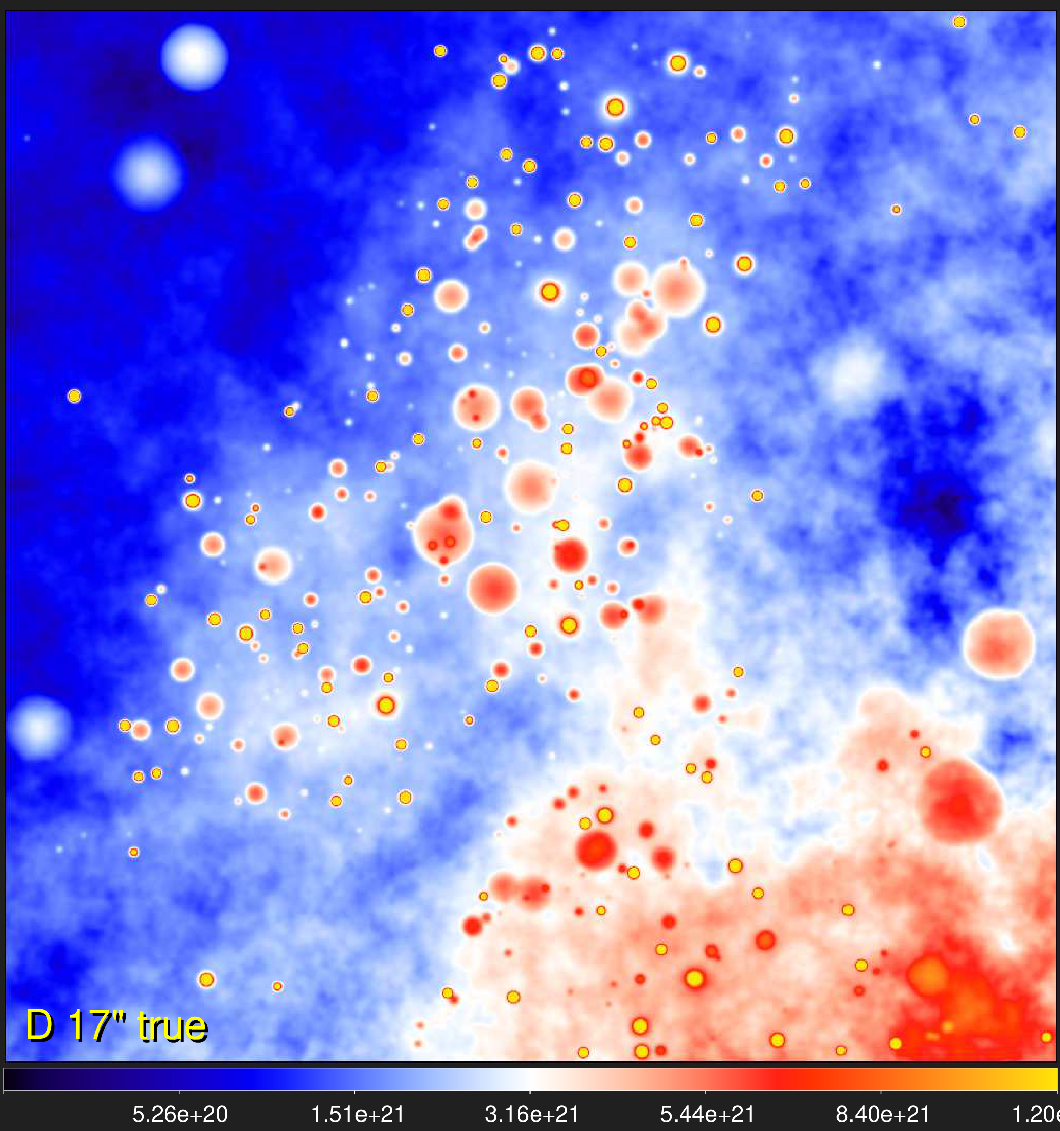
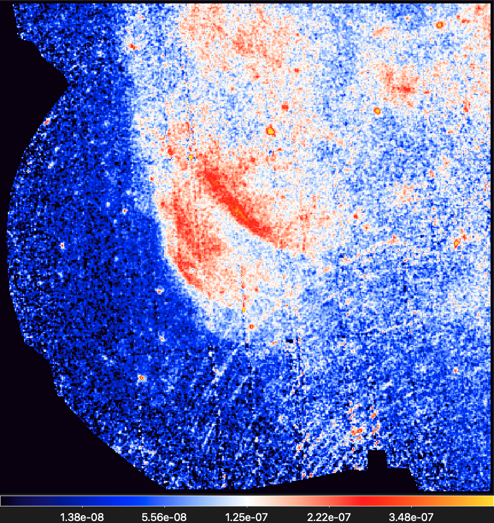
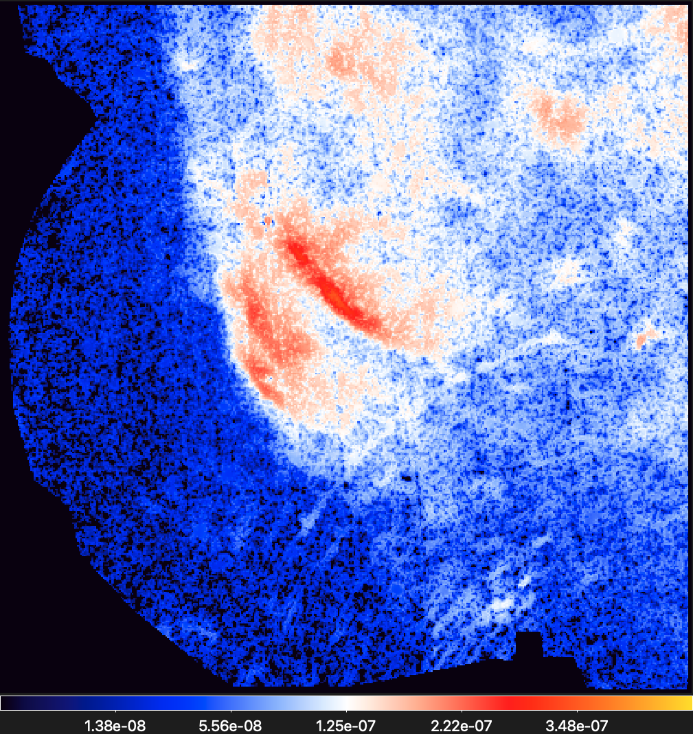
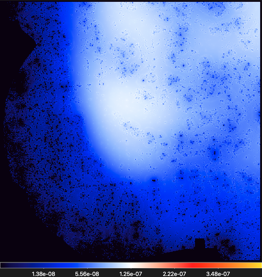
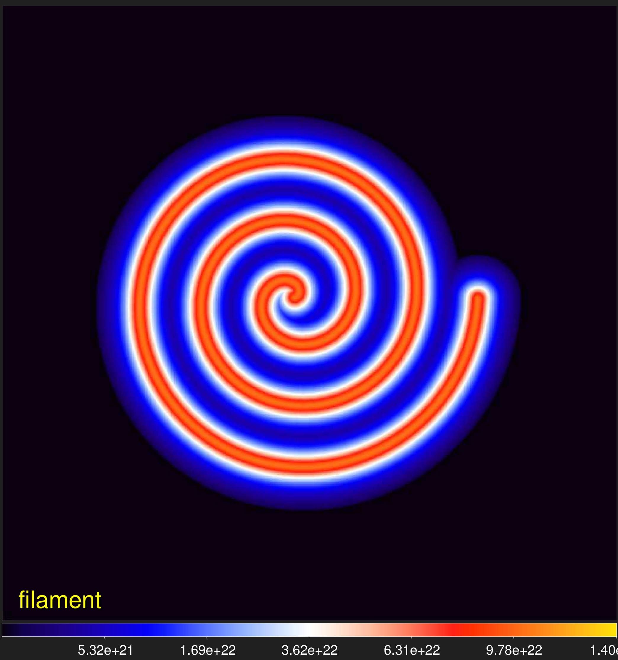
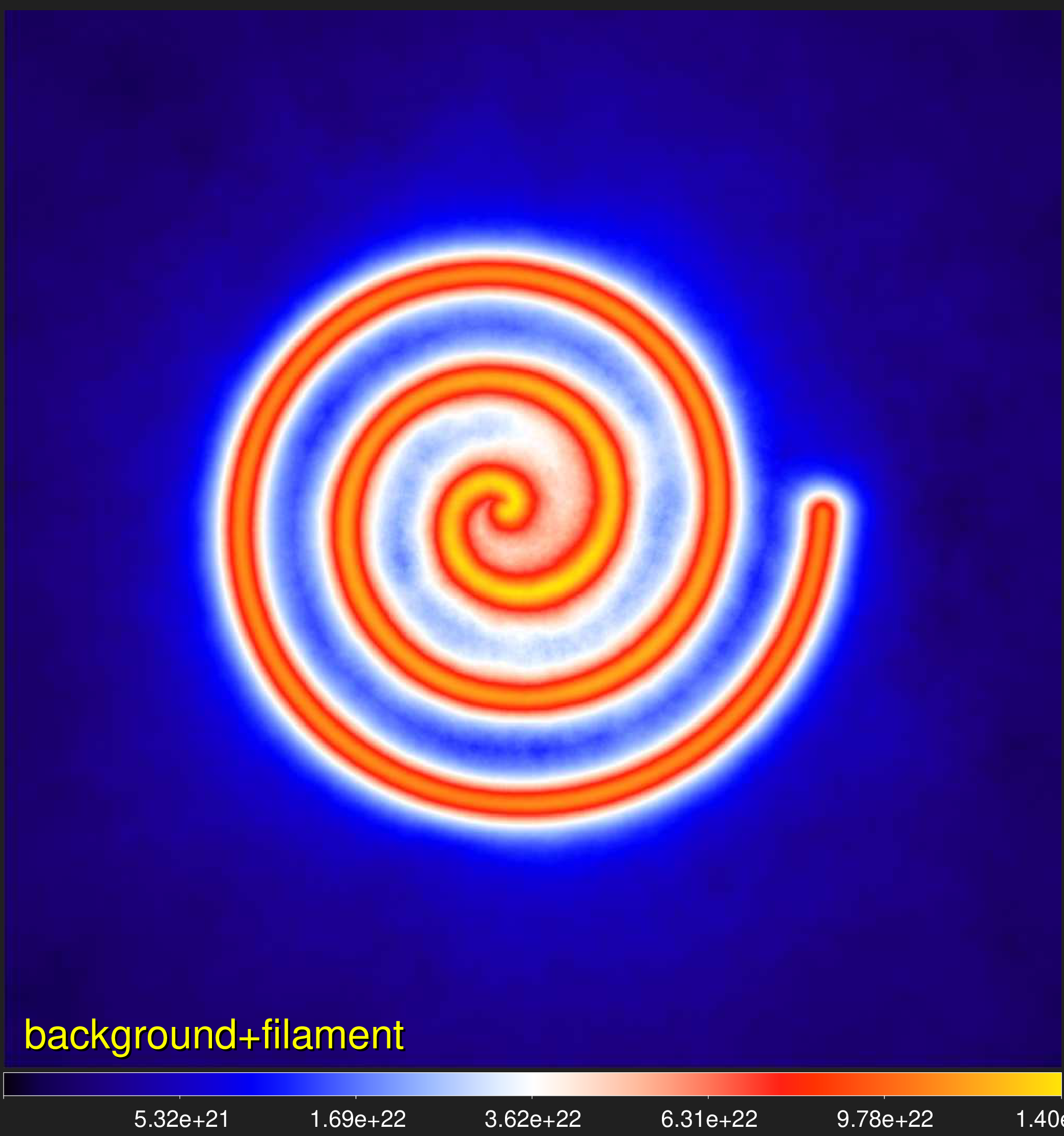
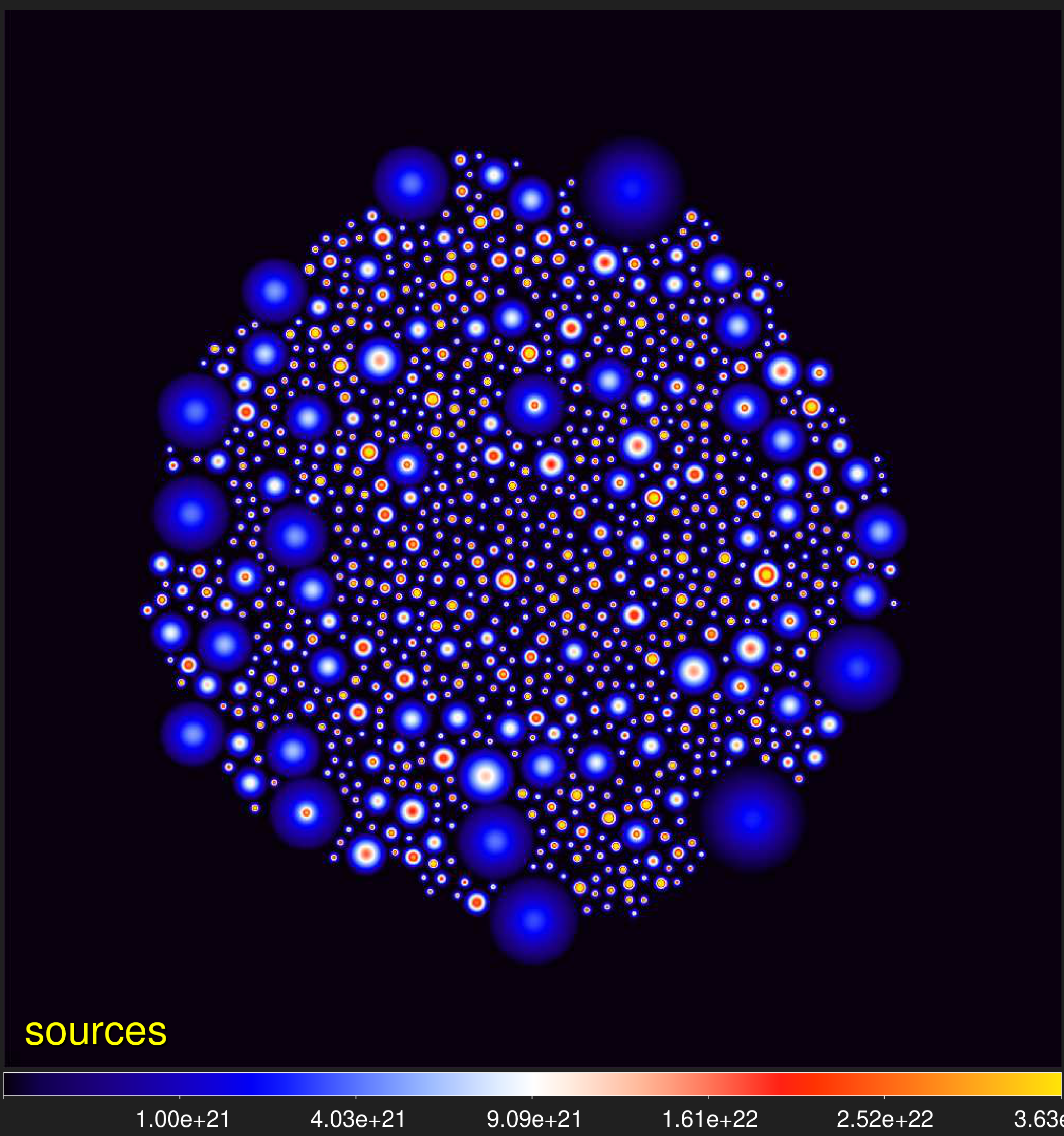
Benchmark B
The new Benchmark B, created by Men'shchikov (2021)
to develop getsf, features a dense and highly variable background cloud, a dense spiral
filament with its markedly anisotropic properties, 919 sources with a wide range of fluxes, sizes, and intensity profiles, and uniform
noise. In contrast to Benchmark A, the sources do not overlap. Benchmark
B with 4 components (background, filament, sources, and noise) is referred to as
B4. Simpler variants include B3
(no filament) and B2 (no filament, no background).
The simplest Benchmark B2 must not present any problems to those extraction methods
that do not set any upper limit on sizes of extractable sources and do not assume Gaussian shapes of their intensity profiles. Only
the faintest sources are expected to be lost within the noise fluctuations in B2
and measurements of sources are expected to be accurate, although for the faintest sources inaccuracies must somewhat increase due
to the noise fluctuations.
The more complex Benchmark B3 could present serious problems to those extraction
methods that are not explicitly designed to handle complex backgrounds. The background fluctuations are strongly nonuniform and they
progressively increase in the denser background area, resembling the observed clouds. In comparison with
B2, this means that more of the sources are expected to remain undetected in
B3 and possibly more spurious sources to become cataloged.
The most complex Benchmark B4 with the dense filamentary background better resembles
the extreme complexity of the interstellar clouds revealed by observations, further complicating the source extraction problem. It can be
expected that a larger number of sources would vanish in the background in B4 and that
measurements of the sources would become less accurate than in the simpler B3 and B2.
The compressed archives below contain the simulated images at 70,
100, 160, 250,
350, and 500 μm (resolutions of
8.4, 9.4, 13.5,
18.2, 24.9, and 36.3"),
the surface density images (resolution of 13.5"), and the truth catalogs with parameters of
all model sources. The archives were produced with rar, because this
compression utility creates the smallest archives of 180, 130, and 120 MB, respectively.
Background
Filament
Background+Filament
Sources
Background+Filament+Sources

< Code
Support >
")
Support
The author supports getsf users and helps them get started, with the usual response
times ranging from minutes to hours. Please note that the code may become updated in the future and that only the
latest version of getsf is supported.
It is strongly recommended that users read the User's Guide containing essential information that would
help them install and use the tool correctly.
If apparently abnormal results are found or the code aborts for unknown reasons, the user is asked to install the latest version
of the code and restart the problematic run from the nearest (previous) processing step to verify that the problem persists. If
the user needs assistance in finding reasons of the problems, the author expects receiving a clear description of the problem, a
copy or screenshot of the contents of the terminal window, and the log files of the runs. In rare cases, it may also be necessary
to re-run the problematic extraction with an updated version.
GETSF In Publications
-
Nony T., Robitaille J.-F., Motte F., et al. (2021) A&A, 645, A94
-
Men'shchikov A. (2021) A&A, 649, A89
(getsf method)
-
Schuller F., André Ph., Shimajiri Y., et al. (2021) A&A, 651, A36
-
Louvet F., Hennebelle P., Men'shchikov A., et al. (2021) A&A, 653, A157
-
Men'shchikov A. (2021) A&A, 654, A78
(getsf benchmarking)
-
Motte F., Bontemps S., Csengeri T., et al. (2022) A&A, 662, A8
-
Kumar M. S. N., Arzoumanian D., Men'shchikov A., et al. (2022)
A&A, 658, A114
-
Pouteau Y., Motte F., Nony T., et al. (2022) A&A, 664, A26
-
Arzoumanian D., Russeil D., Zavagno A., et al. (2022) A&A, 660, A56
-
Zhang C., Zhang G.-Y., Li J.-Z., et al. (2022) RAA, 22, 5, 055012
-
Bhadari N. K., Dewangan L. K., Ojha D. K., et al. (2022) ApJ, 930, 169
-
Thomasson B., Joncour I., Moraux E., et al. (2022) A&A, 665, A119
-
Maity A. K., Dewangan L. K., Sano H., et al. (2022) ApJ, 934, 2
-
Hwang J., Kim J., Pattle K., et al. (2022) ApJ, 941, 51
-
Xu F.-W., Wang K., Liu T., et al. (2023) MNRAS, 520, 3259
-
Dewangan L. K., Bhadari N. K., Men'shchikov A., et al. (2023) ApJ, 946, 22
-
Dewangan L. K., Bhadari N. K., Maity A. K., et al. (2023) JOAA, 44, 23
-
Padoan P., Pelkonen V-M., Juvela M., et al. (2023) MNRAS, 522, 3548
-
Pouteau Y., Motte F., Nony T., et al. (2023) A&A, 674, 76
-
Nony T., Galvan-Madrid R., Motte F., et al. (2023) A&A, 674, 75
-
Li, X.-M., Zhang G.-Y., Men'shchikov A., et al. (2023) A&A, 674, 225
-
Men'shchikov A., (2023) A&A, 675, 185
-
Maity A. K., Dewangan L. K., Bhadari N. K., et al. (2023) MNRAS, 523, 5388
-
Mookerjea B., Sandell G., Guesten, R., et al. (2023) MNRAS, 525, 5468
-
Seshadri A., Vig S., Ghosh S. K., et al. (2024) MNRAS, 527, 4244
-
Dewangan L. K., Bhadari N. K., Maity A. K., et al. (2024) MNRAS, 527, 5895
-
Xu F., Wang K., Liu T., et al. (2024) ApJS, 270, 9
-
Armante M., Gusdorf A., Louvet F., et al. (2024) A&A, 686, 22
-
Cheng Y., Lu X., Sanhueza P., et al. (2024) ApJ, 967, 56
-
Dell'Ova P., Motte F., Gusdorf A., et al. (2024) A&A, 687, 217
-
Nony T., Galvan-Madrid R., Brouillet N., et al. (2024) accepted
-
Zhang G., André Ph., Men'shchikov A. (2024) A&A, accepted
-
Bonfand M., Csengeri T., Bontemps S., et al. (2024) A&A, accepted
-
Louvet F., Sanhueza P., Stutz A., et al. (2024) A&A, submitted
< Bench
Intro >
")
Elements
Text
This is bold and this is strong. This is italic and this is emphasized.
This is superscript text and this is subscript text.
This is underlined and this is code: for (;;) { ... }. Finally, this is a link.
Heading Level 2
Heading Level 3
Heading Level 4
Heading Level 5
Heading Level 6
Blockquote
Fringilla nisl. Donec accumsan interdum nisi, quis tincidunt felis sagittis eget tempus euismod.
Vestibulum ante ipsum primis in faucibus vestibulum. Blandit adipiscing eu felis iaculis volutpat
ac adipiscing accumsan faucibus. Vestibulum ante ipsum primis in faucibus lorem ipsum dolor sit amet
nullam adipiscing eu felis.
Preformatted
i = 0;

while (!deck.isInOrder()) {
    print 'Iteration ' + i;
    deck.shuffle();
    i++;
}

print 'It took ' + i + ' iterations to sort the deck.';
Lists
Unordered
- Dolor pulvinar etiam.
- Sagittis adipiscing.
- Felis enim feugiat.
Alternate
- Dolor pulvinar etiam.
- Sagittis adipiscing.
- Felis enim feugiat.
Ordered
- Dolor pulvinar etiam.
- Etiam vel felis viverra.
- Felis enim feugiat.
- Dolor pulvinar etiam.
- Etiam vel felis lorem.
- Felis enim et feugiat.
Icons
Actions
Table
Default
| Name |
Description |
Price |
| Item One |
Ante turpis integer aliquet porttitor. |
29.99 |
| Item Two |
Vis ac commodo adipiscing arcu aliquet. |
19.99 |
| Item Three |
Morbi faucibus arcu accumsan lorem. |
29.99 |
| Item Four |
Vitae integer tempus condimentum. |
19.99 |
| Item Five |
Ante turpis integer aliquet porttitor. |
29.99 |
|
100.00 |
Alternate
| Name |
Description |
Price |
| Item One |
Ante turpis integer aliquet porttitor. |
29.99 |
| Item Two |
Vis ac commodo adipiscing arcu aliquet. |
19.99 |
| Item Three |
Morbi faucibus arcu accumsan lorem. |
29.99 |
| Item Four |
Vitae integer tempus condimentum. |
19.99 |
| Item Five |
Ante turpis integer aliquet porttitor. |
29.99 |
|
100.00 |