(...) the Bayesian method is easier to apply and yields the same or better
results. (...) the orthodox results are satisfactory only when they agree
closely (or exactly) with the Bayesian results. No contrary example has
yet been produced. (...) We conclude that orthodox claims of superiority
are totally unjustified; today, the original statistical methods of Bayes
and Laplace stand in a position of proven superiority in actual
performance, that places them beyond the reach of mere ideological or
philosophical attacks. It is continued teaching and use of orthodox
methods that is in need of justification and defense.
(Edwin T. JAYNES; Jaynes, 1976)
We have stressed earlier that ISD studies were essentially empirical, because of the complexity of their subject. Most of the time, they consist in interpreting data with formulae and models. Yet, comparing observations to models is a very wide methodological topic. It also has epistemological 1 consequences. All the knowledge we derive about ISD depends on the way it was inferred. The question of the methods we use, and the way we articulate different results to build a comprehensive picture of the ISM, is thus of utmost importance.
Historically, two competitive visions of the way empirical data should be quantitatively compared to models have emerged, the (i) Bayesian, and (ii) frequentist methods. We personally follow the Bayesian method and will try to give arguments in favor of its superiority. An efficient way to present the Bayesian approach is to compare it to its alternative, and to show how both methods differ. There is a large literature on the subject. The book of Gelman et al. (2004) is a reference to learn Bayesian concepts and techniques. The posthumous book of Jaynes (2003) is more theoretical, but very enlightening. Otherwise, several reviews have been sources of inspiration for what follows (Jaynes, 1976; Loredo, 1990; Lindley, 2001; Bayarri & Berger, 2004; Wagenmakers et al., 2008; Hogg et al., 2010; Lyons, 2013; VanderPlas, 2014). A good introduction to frequentist methods can be found in the books of Barlow (1989) and Bevington & Robinson (2003).
Bayesian and frequentist methods differ by: (i) the meaning they attribute to probabilities; and (ii) the quantities they consider random. Their radically different approaches and the various bifurcations the two methods take to address a given problem originate from these sole conceptions.
The concept of conditional probability is central to what follows. As we will see, Bayesian and frequentist approaches differ on this aspect.
The meaning of conditional probabilities. If and are two logical propositions, the conditional probability, noted , is the probability of being true, knowing is true. To give an astronomical example, let’s assume that:
Since most stars are LIMS, and that they have a lifetime Gyr, we can estimate the probability to observe a SN Ia, knowing we are observing a binary system:
| (5.1) |
On the contrary the probability to observe a binary system, knowing we are observing a SN Ia is:
| (5.2) |
because SN Ia happen only in binary systems. We see that . In our example, the two quantities do not even have the same units.
All probabilities are conditional. In practice, all probabilities are conditional. In the previous example, we have implicitly assumed that our possibility space, that is the ensemble of cases we can expect out of the experiment we are conducting, contained all the events where we are actually observing a star, when we are pointing our telescope at its coordinates. However, what if there is suddenly a cloud in front of the telescope? We would then need to account for these extra possibilities, which is equivalent to adding conditions. For instance, if we are conducting the same experiment from a ground-based telescope in London, during winter, we will get:
| (5.3) |
where the symbol denotes the logical “and”.
All probabilities are conditional and the possible conditions are limited by our own knowledge.
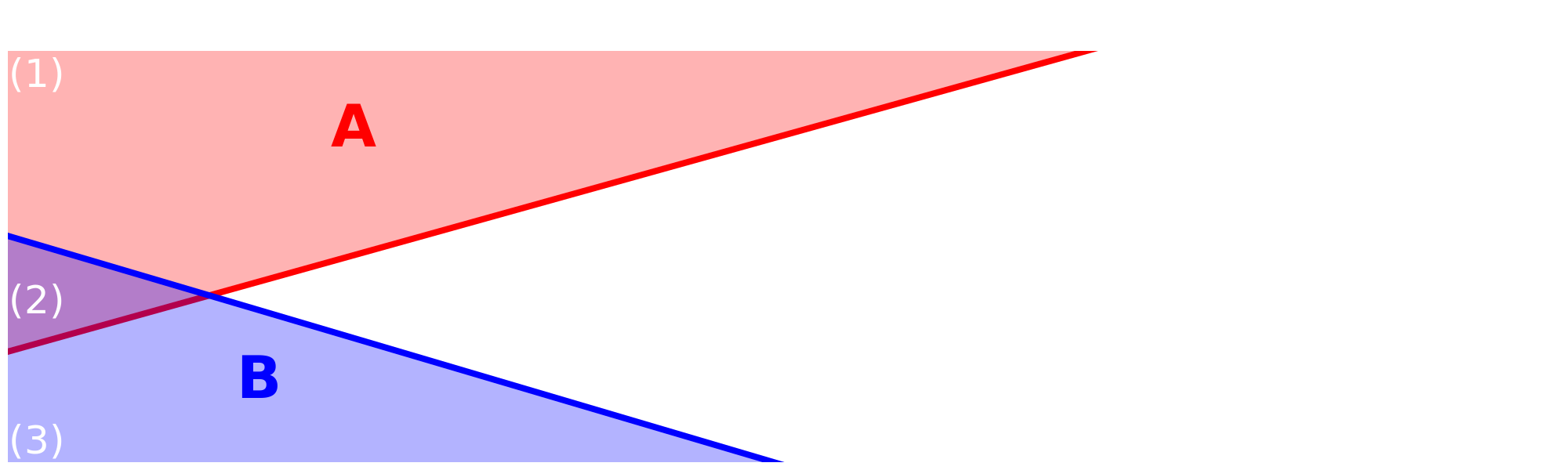
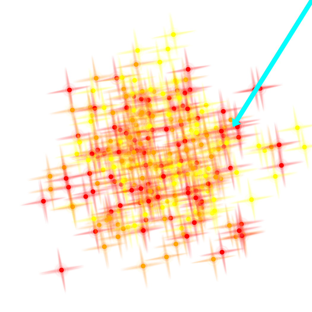
Bayes’ rule. Thomas BAYES derived, in the middle of the XVIII century, a formula to reverse the event and the condition, in conditional probabilities. Fig. 5.1 shows a Venn diagram, that is a graphic representation of a possibility space. We have shown an arbitrary event A, in red, and another event B, in blue. The intersection of A and B, numbered (2), can be written . The probability of A, knowing B, is the probability of A, when B is considered as the new possibility space. In other words:
| (5.4) |
We therefore have: . By symmetry of A and B, we have , thus , which gives Bayes’ rule:
| (5.5) |
We review here the assumptions of both methods, in a general, abstract way. We will illustrate this presentation with concrete examples in Sect. 5.1.2. Let’s consider we are trying to estimate a list of physical parameters, , using a set of observations, . Let’s also assume that we have a model, , predicting the values of the observables, , for any value of : .
The Bayesian viewpoint. The Bayesian approach considers that there is an objective truth, but that our knowledge is only partial and subjective. Bayesians thus assume the following.
| (5.6) |
Compared to Eq. (), Eq. () misses the denominator, . This is because this distribution is independent of our variables, that are the physical parameters. If we were to explicit it, it would be:
| (5.7) |
which is simply the normalization factor of . This factor can thus be estimated by numerically normalizing the posterior, hence the proportionality we have used in Eq. (). The three remaining terms are the following.
| (5.8) |
The frequentist viewpoint. The frequentist approach also considers that there is an objective truth, but it differs with the Bayesian viewpoint by rejecting its subjectivity. Frequentists thus assume the following.
Bayesians do not tamper with the data, whereas frequentists account for hypothetical data that have not actually been obtained.
We now compare the two approaches on a series of simple examples, in order to demonstrate in which situations the two approaches may differ.
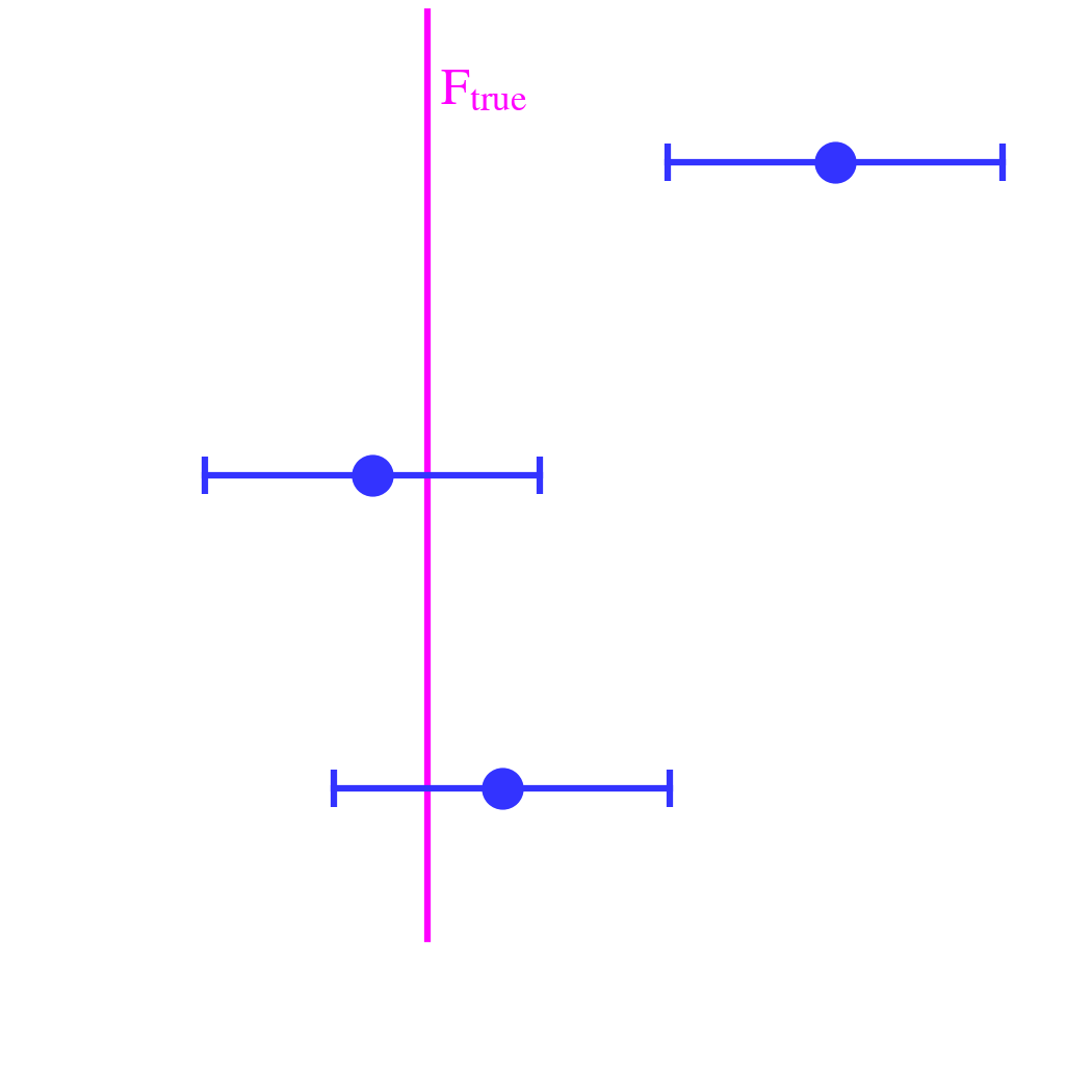
Let’s assume we are trying to estimate the flux of a star, , in a given photometric filter, with the following assumptions.
This is represented in Fig. 5.2. There is an analytic solution to this simple case:
| (5.9) |
 |  |
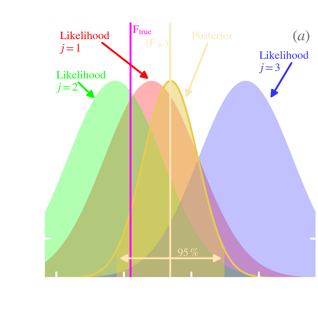
The Bayesian solution. The Bayesian solution is obtained by sampling the posterior distribution in Eq. (): .
| (5.10) |
The solution is represented in Fig. 5.3.a. We have sampled the posterior using a Markov Chain Monte-Carlo method (MCMC; using the code emcee by Foreman-Mackey et al., 2013). We will come back to MCMC methods in Sect. 5.1.3. The estimated value is ( uncertainty). This is exactly the analytical solution in Eq. (). The credible range, that is the range centered on containing a probability, is .
 |  |
The frequentist solution. There are different ways to approach this problem in the frequentist tradition. The most common solution would be to use a Maximum-Likelihood Estimation (MLE) method.
A few remarks. We can see that both methods give the same exact result, which is also consistent with the analytical solution (Eq. ). This is because the assumptions were simple enough to make the two approaches equivalent:
Note also our subtle choice of terminology: (i) we talk about credible range in the Bayesian case, as this term designates the quantification of our beliefs; while (ii) we talk about confidence interval in the frequentist case, as it concerns our degree of confidence in the results, if the experiment was repeated a large number of times, assuming the population mean is the maximum likelihood.
A first way to find differences between the Bayesian and frequentist approaches is to explore the effect of the prior. To that purpose, let’s keep the same experiment as in Sect. 5.1.2.1, but let’s assume now that the star we are observing belongs to a cluster, and we know its distance.
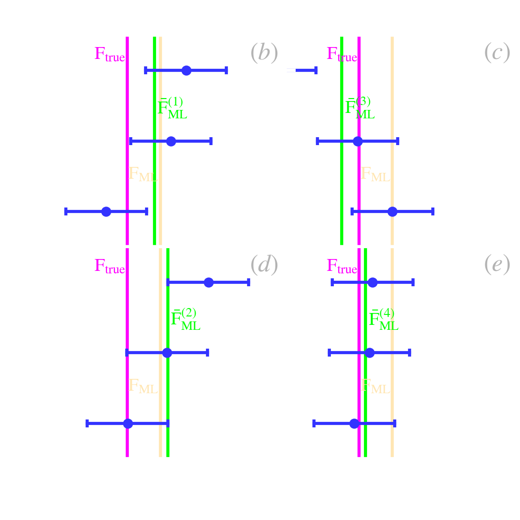
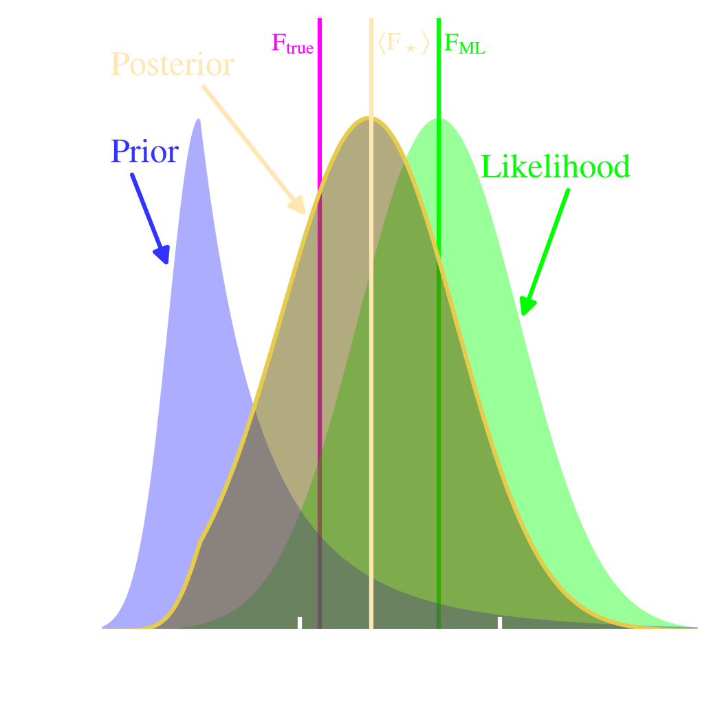
The Bayesian improvement. Contrary to Sect. 5.1.2.1, where we had to guess a very broad, flat prior, we can now refine this knowledge, based on the expected luminosity function, scaled at the known distance of the cluster. This is represented on Fig. 5.4. The posterior distribution (yellow) is now the product of the likelihood (green) and prior (blue). The frequentist solution has not changed, as it can not account for this kind of information. We can see that the maximum a posteriori is now closer to the true value than the maximum likelihood. This can be understood the following way.
If we perform several such measures, there will be some Bayesian solutions that will get corrected farther away from the true flux. This is a consequence of stochasticity. On Fig. 5.4, keeping our value of , this will be the case if the noise fluctuation, is negative, that is if the observed flux is lower than (). However, this deviation will be less important than the correction we would benefit from if the same fluctuation was positive, because the prior would be higher: (cf. Fig. 5.4). The prior would therefore correct less the likelihood on the left side, in this particular case. Thus, on average, taking into account this informative prior will improve the results.
 |  |
Accumulation of data. In this case and the previous one (Sect. 5.1.2.1), we had three observations of the same flux. The posterior distribution we sampled was:
| (5.11) |
This is because we considered the three measures as part of the same experiment. However, we could have chosen to analyze the data as they were coming. After the first flux, we would have inferred:
| (5.12) |
This posterior would have been wider (i.e. more uncertain), as we would have had only one data point. Note that such an inference would have not been possible with a frequentist method, as we would have had one parameter for one constraint (i.e. zero degree of freedom). What is interesting to note is that the analysis of the second measure, can be seen as taking into account the first measure in the prior:
| (5.13) |
and so on. For the third measure, the new prior would be :
| (5.14) |
which is formally equivalent to Eq. (), but is a different way of looking at the prior. Notice that the original prior, , appears only once in the product. The more we accumulate data, the less important it becomes.
The Bayesian approach is an optimal framework to account for the accumulation of knowledge.
The other reason why the two approaches might differ is because Bayesians sample , whereas frequentists produce a series of tests based on . The difference becomes evident when we consider non-Gaussian errors with small data sets.
Flux with a non-linear detector. Let’s assume that we are measuring again the flux from the same star (), with repetitions, but that our detector is now highly non-linear. This non-linearity translates into a heavily-skewed split-normal noise distribution (cf. Sect. C.2.2):
| (5.15) |
with and . This noise distribution is the red curve in Fig. 5.5.a. In practice, this could for example be a very accurate detector suffering from transient effects. The measured value would be systematically higher than the true flux 4. We have simulated three such measures in Fig. 5.5.a, in blue. This problem was adapted from example 5 of Jaynes (1976).
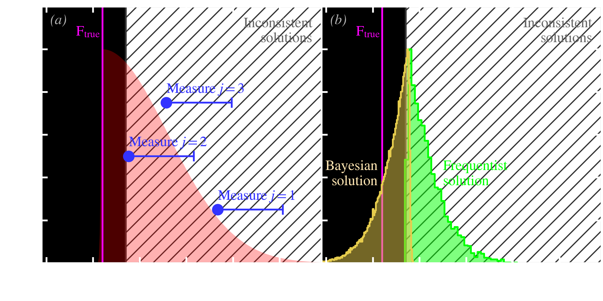
The solutions. Knowing that the measured flux is always greater than or equal to the true flux, it is obvious that the solution should be lower than the lowest measured flux: , in our particular case. This flux range, corresponding to inconsistent values, has been hatched in grey, in Fig. 5.5.
When increases, the frequentist solution gets closer and closer to the true flux. However, a bootstrapping analysis will reject the true flux in of the cases.
The reason of the frequentist failure. The failure of the frequentist approach is a direct consequence of its conception of probability (cf. e.g. VanderPlas, 2014, for a more detailed discussion and more examples). The frequentist method actually succeeds in returning the result it pretends to give: predicting a confidence interval where the solution would fall 95 % of the time, if we repeated the same procedure a large number of times. This is however not equivalent to giving the credible range where the true value of the parameter has a 95 % probability to be (the Bayesian solution). With the frequentist method, we have no guarantee that the true flux will be in the confidence interval, only the solution. We can see that the main issue with the frequentist approach is that it is difficult to interpret, even in a simple problem such as that of Fig. 5.5. “Bayesians address the question everyone is interested in by using assumptions no-one believes, while Frequentists use impeccable logic to deal with an issue of no interest to anyone” (Lyons, 2013). In the previous citation, the “assumption no-one believes” is the subjective choice of the prior, and the “issue of no interest to anyone” is the convoluted way frequentists formulate a problem, to avoid assigning probabilities to parameters.
Frequentist results can be inconsistent in numerous practical applications, and they never perform better than Bayesian methods.
Bayesian problems are convenient to formulate as they consist in laying down all the data, the model, the noise sources and the nuisance variables to build a posterior, using Bayes’ rule. The Bayesian results are also convenient to interpret as they all consist in using the posterior, which gives the true probability of the parameters. However, in between, estimating the average, standard deviation, correlation coefficients of parameters, or testing hypotheses can be challenging, especially if there are a lot of parameters or if the model is complex. Fortunately, several numerical methods have been introduced to make these tasks simpler. Most of these methods are based on Markov Chain Monte-Carlo (MCMC 5), which are a class of algorithms for sampling PDFs.
Markov Chains Monte-Carlo. A MCMC draws samples from the posterior. In other words, it generates a chain of values of the parameters, (). These parameter values are not uniformly distributed in the parameter space, but their number density is proportional to the posterior PDF. Consequently, there are more points where the probability is high, and almost none where the probability is low. It has several advantages.
| (5.16) |
where the second equality is simply the average of the sample. We could do the same for the standard deviation, or the correlation coefficient.
All these operations would have been much more expensive, in terms of computing time, if we had to numerically solve the integral. In particular, computing the normalization of the whole posterior would have been costly. From a technical point of view, a MCMC is a random series of values of a parameter where the value at step depends only the value at step . We briefly discuss below the two most used algorithms. A good presentation of these methods can be found in the book of Gelman et al. (2004) or in the Numerical recipes (Press et al., 2007).
The Metropolis-Hastings algorithm. To illustrate this method and the next one, let’s consider again the measure of the flux of our star, with the difference, this time, that we would be observing it through two different photometric filters.
| (5.17) |
The posterior is thus, noting and :
| (5.18) |
Contours of this distribution are represented in Fig. 5.6.a-b.
The algorithm proposed by Metropolis et al. (1953) and generalized by Hastings (1970) is the most popular method to sample any PDF. This is a rejection method, similar to what we have discussed for MCRTs, in Sect. 3.1.1.4 (cf. also Appendix C.2.3.1).
| (5.19) |
| (5.20) |
The function is here to make sure we get a result between 0 and 1. In our case, we have chosen a symmetric proposal distribution. Eq. () thus implies that:
| (5.21) |
We just need to estimate our posterior at one position (assuming we saved the value of , after the previous iteration). In addition, since we need only the ratio of two points in the posterior, we do not need to normalize it. This is the reason why this algorithm is so efficient.
The initial value of the chain has to be a best guess.
The sampling of Eq. () with the Metropolis-Hastings method is shown in Fig. 5.6.a.
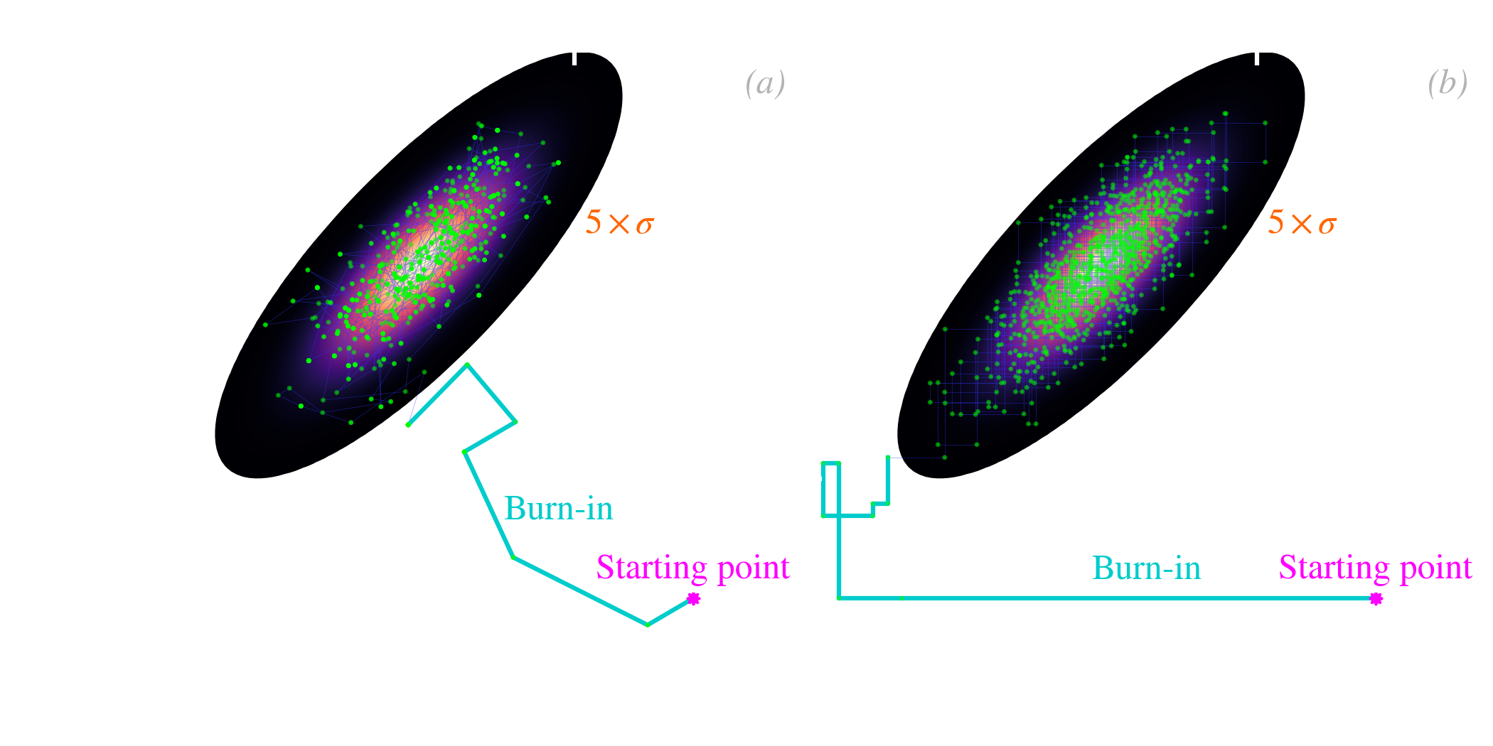
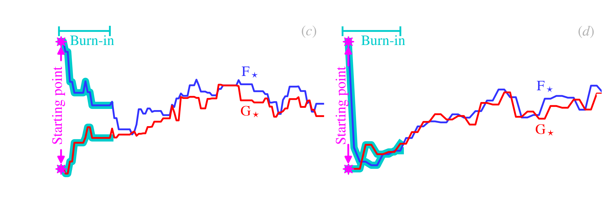
Gibbs sampling. The number of parameters, , determines the dimension of the posterior. The higher this number is, the smaller the support of the function is (i.e. the region where the probability is non negligible). Metropolis-Hastings methods therefore will have a high rejection rate, if , requiring longer chains to ensure convergence. Gibbs sampling (Geman & Geman, 1984) provides an alternative MCMC method, where all draws are accepted. Its drawback is that it requires normalizing, at each iteration, the full conditional distribution:
| (5.22) |
that is the posterior fixing all parameters except one. This is only a one dimensional PDF, though, much less computing-intensive than the whole posterior. The method consists, at each iteration , to cycle through the different parameters, and draw a new value from Eq. ():
| (5.23) |
Since this distribution has an arbitrary form, random drawing can be achieved numerically using the CDF inversion method (Appendix C.2.3.2). Fig. 5.6.b represents the Gibbs sampling of Eq. (). The squared pattern comes from the fact that we alternatively sample each parameter, keeping the other one fixed.
Assessing convergence. One of the most crucial questions, when using a MCMC method, is how long a chain do we need to run. To answer that question, we need to estimate if the MCMC has converged toward the stationary posterior. Concretely, it means that we want to make sure the sampling of the posterior is homogeneous, and that the moments and hypothesis testing we will perform will not be biased, because some areas of the parameter space have only been partially explored. The reason why the sampling of the parameter space might be incomplete is linked to the two following factors.
| (5.24) |
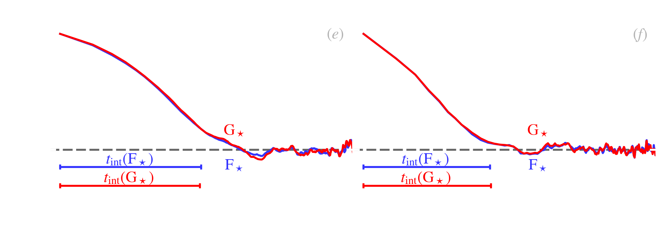
This is the correlation coefficient of the parameter with itself, shifted by steps. The ACFs of our example are displayed in Fig. 5.6.e-f. We can see that the ACF starts at 1, for . It then drops over a few steps and oscillates around 0. The typical lag after which the ACF has dropped to 0, corresponds to the average number of steps necessary to draw independent values. This typical lag can be quantified, by the integrated autocorrelation time, 6:
| (5.25) |
It is represented in Fig. 5.6.e-f. It corresponds roughly to the average number of steps needed to go from one end of the posterior to the other. Different parameters of a given MCMC can in principle have very different (e.g. Galliano, 2018). To make sure that our posterior is properly sampled, we thus need to let our MCMC run a large number of steps, times , after burn-in. The effective sample size, , quantifies the effective number of steps that can be considered independent. We need .
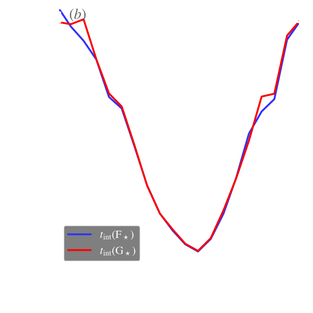
With the Metropolis-Hastings algorithm, the integrated autocorrelation time will depend heavily on the choice of the proposal distribution. We have explored the effect of the width of this distribution on . In Eq. (), instead of taking and , we have varied this parameter. Fig. 5.7.a represents the mean rejection rate as a function of .
Fig. 5.7.b shows that the only range where is reasonable is when the width of the proposal distribution is comparable to the width of the posterior.
 |  |
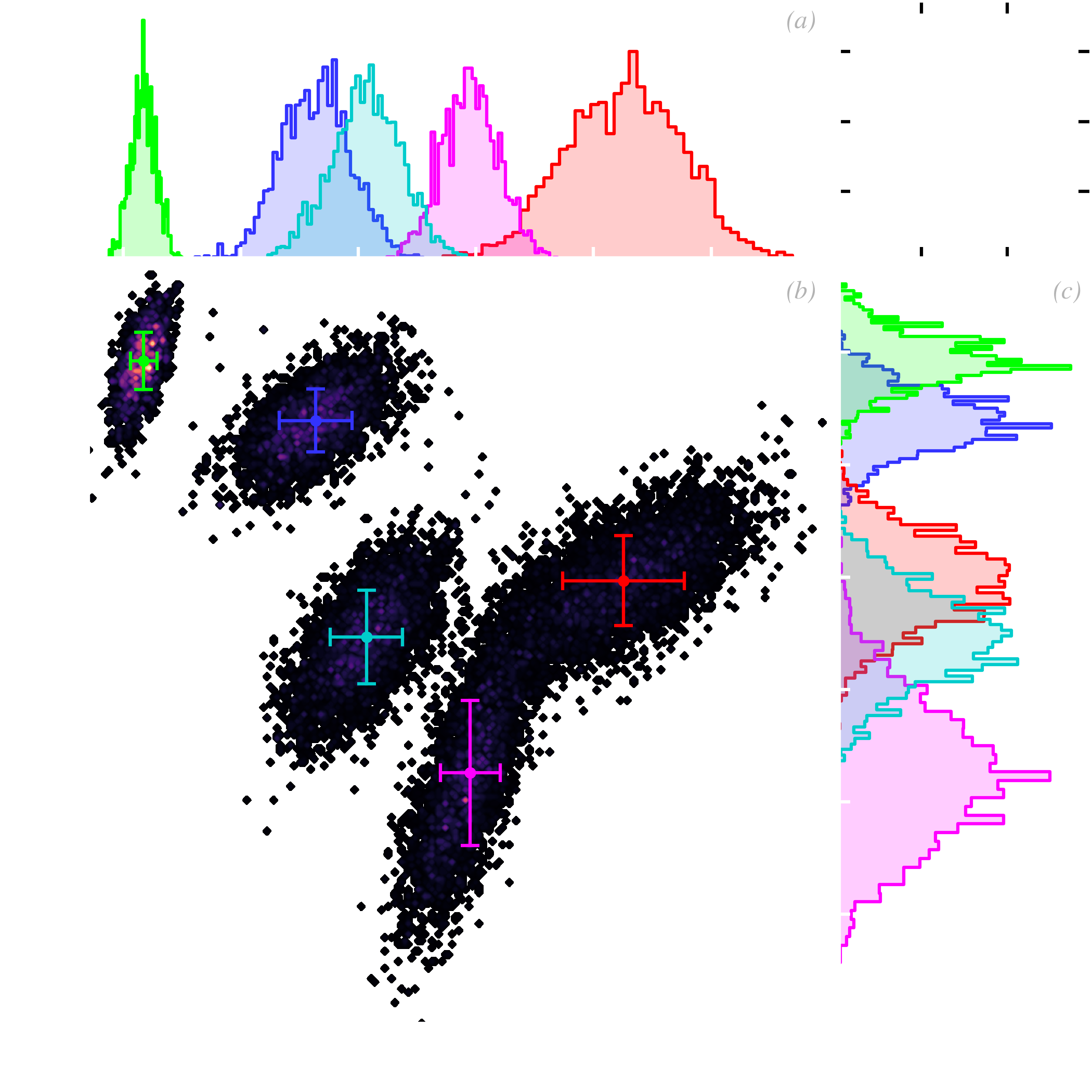
Parameter inference. Numerous quantities can be inferred from a MCMC. We have previously seen that the average, uncertainties, and various tests can be computed using the posterior of the parameters of a source. This becomes even more powerful when we are analyzing a sample of sources. To illustrate this, let’s assume we are now observing stars, through the same photometric bands as before. Fig. 5.8.b shows the posterior PDF of the two parameters of the five stars. It is important to distinguish the following two types of distributions.
| (5.26) |
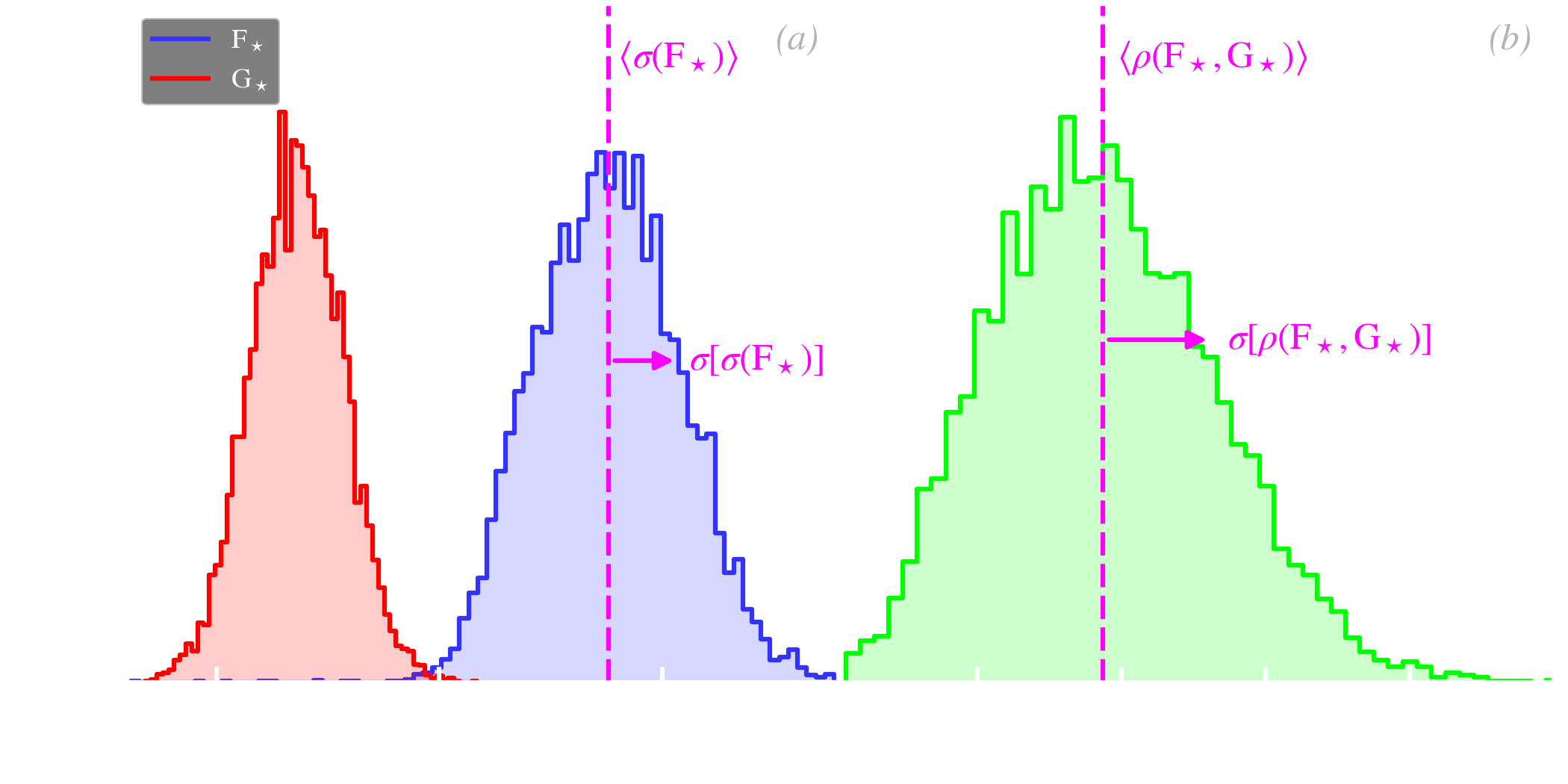
where is the observed flux of the star , at the MCMC iteration . It is how we can quantify the dispersion of the sample. We can thus quote the sample dispersion as (cf. Fig. 5.9.a):
| (5.27) |
In our example, we have: and . We can see that these values correspond roughly to the intrinsic scatter between individual stars, in Fig. 5.8.b, but they are larger than the uncertainty on the flux of individual stars. We can do the same for the correlation coefficient, as shown in Fig. 5.9.b: . Notice that it is negative, because the correlation between stellar fluxes, in Fig. 5.8.b, points toward the lower right corner. However, the correlation between the uncertainties on and is positive: the individual ellipses point in the other direction, toward the upper right corner. We have deliberately simulated data with these two opposite correlations to stress the difference between the individual likelihood properties and those of the ensemble. Finally, we could have done the same type of estimate for the mean of the sample: and .
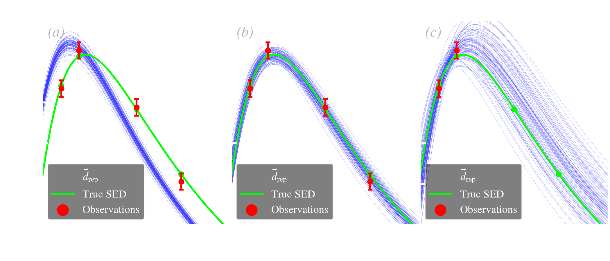
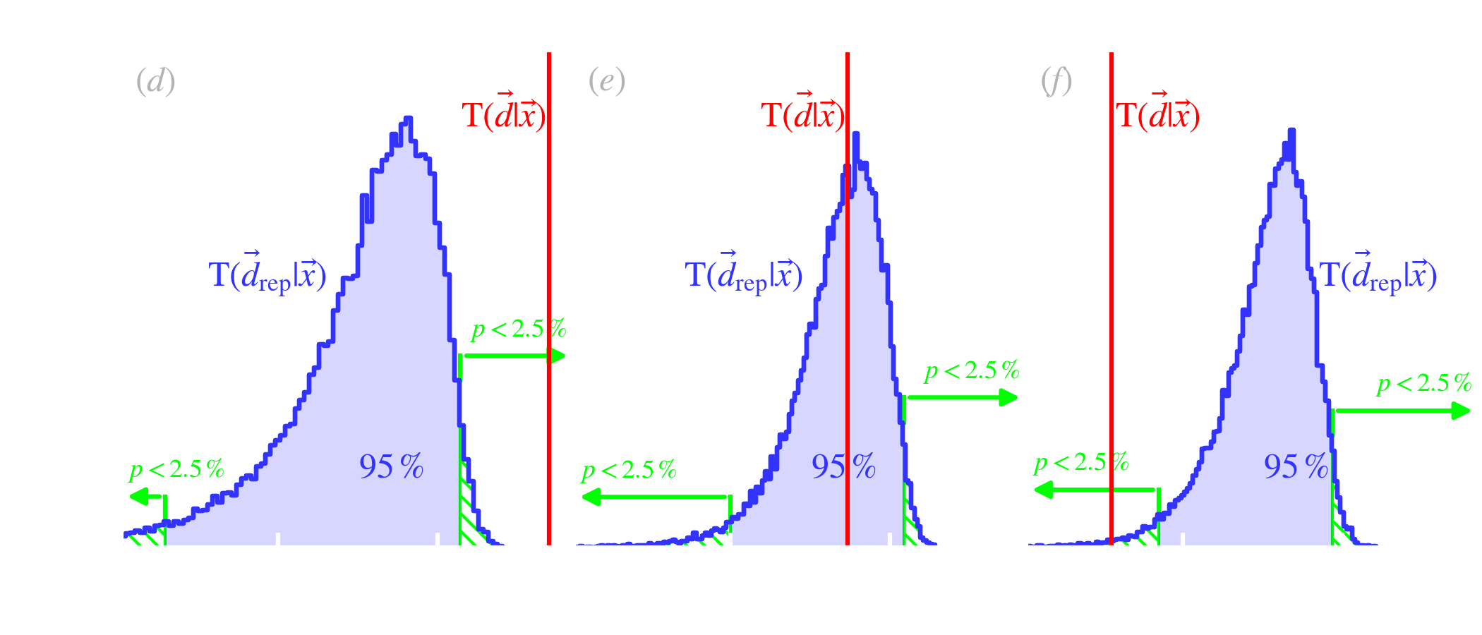
Quantifying the goodness of a fit. It is important, in any kind of model fitting, to be able to assess the quality of the fit. In the frequentist approach, this is done with the chi-squared test, which is limited in its assumptions to normal iid noise, without nuisance parameters. In the Bayesian approach, the same type of test can be done, accounting for the full complexity of the model (non-Gaussian errors, correlations, nuisance parameters, priors). This test is usually achieved by computing posterior predictive -values (ppp; e.g. Chap. 6 of Gelman et al., 2004). To illustrate how ppps work, let’s consider now that we are observing the same star as before, through four bands (R, I, J, H) and are performing a blackbody Bayesian fit to this SED, varying the temperature, , and the dilution factor, . This is represented in Fig. 5.10.b. The principle is the following.
| (5.28) |
If we sampled our posterior with a MCMC, this integral can simply be computed by evaluating our model (the blackbody, in the present case), for values of our drawn parameters: .
| (5.29) |
We compute this quantity both for the replicated set, , which is the blue distribution in Fig. 5.10.e, and for the observations, , which is the red line in Fig. 5.10.e (it is a single value). To be clear, only the data term in Eq. () changes between and . The quantities and are identical in both cases.
| (5.30) |
If the difference between the replicated set and the data is solely due to statistical fluctuations, we should have on average . The fit is considered bad, at the level, if or .
We have illustrated this test in Fig. 5.10, varying the number of parameters and observational constraints, in order to explore the different possible cases.
There is no issue with fitting even fewer constraints than parameters, with a Bayesian approach. The consequence is that the posterior is going to be very wide along the dimensions corresponding to the poorly constrained parameters. However, the results will be consistent, and the derived probabilities will be meaningful.
Contrary to the frequentist approach, we can fit Bayesian models with more parameters than data points.
We now resume our comparison of the Bayesian and frequentist approaches, started in Sect. 5.1.2. We focus more on the interpretation of the results and synthesize the advantages and inconveniences of both sides.
Until now, we have seen how to estimate parameters and their uncertainties. It is however sometimes necessary to be able to make decisions, that is to choose an outcome or its alternative, based on the observational evidence. Hypothesis testing consists in assessing the likeliness of a null hypothesis, noted . The alternative hypothesis is usually noted , and satisfies the logical equation , where the symbol is the logical negation. The priors necessarily obey . To illustrate this process let’s go back to our first example, in Sect. 5.1.2. We are observing a star with true flux , times, with an uncertainty on each individual flux measurements, . This time, we want to know if , for a given .
Bayesian hypothesis testing. Bayesian hypothesis testing consists in computing the posterior odds of the two complementary hypotheses:
| (5.31) |
The posterior odds is the ratio of the posterior probabilities of the two hypotheses. It is literally the odds we would use for gambling (e.g. a posterior odd of 3 corresponds to a 3:1 odd in favor of ). The important term in Eq. () is the Bayes factor, usually noted . It quantifies the weight of evidence, brought by the data, against the null hypothesis. It tells us how much our observations changed the odds we had against , prior to collecting the data. Table 5.1 gives a qualitative scale to decide upon Bayes factors. We see that it is a continuous credibility range going from rejection to confidence. The posterior of our present example, assuming a wide flat prior, is:
| (5.32) |
where . The posterior probability of is then simply:
| (5.33) |
It is represented in Fig. 5.11.a. This PDF is centered in , since, as usual in the Bayesian approach, it is conditional on the data. Fig. 5.11.a shows the complementary posteriors of (red) and (blue), which are the incomplete integrals of the PDF. When we vary , the ratio of the two posteriors, , changes. Assuming we have chosen a very wide, flat prior, such that , the Bayes factor becomes:
| (5.34) |
Fig. 5.11.b represents the evolution of the Bayes factor as a function of the sample size, . In this particular simulation, is false. We see that, when increases, we accumulate evidence against , going through the different levels of Table 5.1. The evidence is decisive around , here.
| Bayes factor, BF | Strength of evidence against H |
| 1–3.2 | Barely worth mentioning |
| 3.2–10 | Substantial |
| 10–32 | Strong |
| 32–100 | Very strong |
| >100 | Decisive |
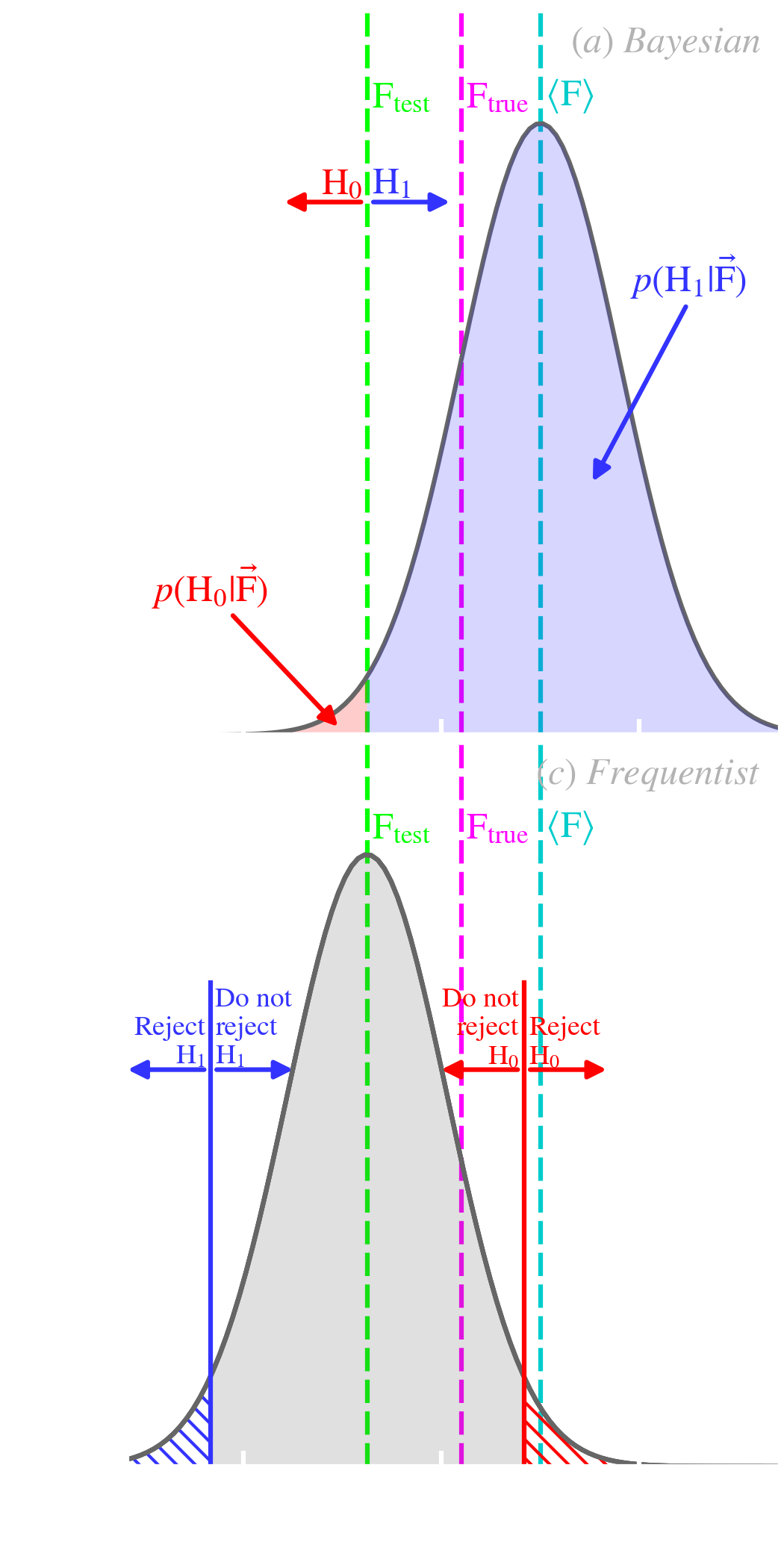 | 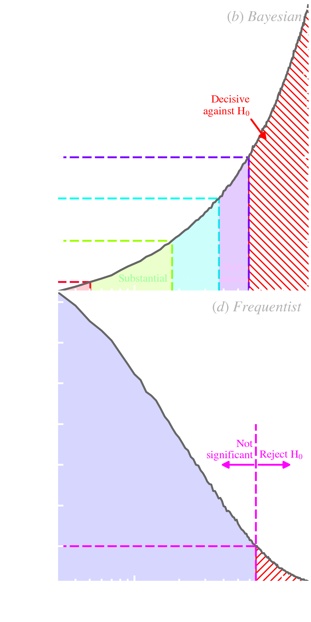 |
Frequentist hypothesis testing. Instead of computing the credibility of against , the frequentist approach relies on the potential rejection of . It is called Null Hypothesis Significance Test (NHST; e.g. Ortega & Navarrete, 2017). It consists in testing if the observation average, , could have confidently been drawn out of a population centered on . In that sense, it is the opposite of the Bayesian case. This is demonstrated in Fig. 5.11.c. We see that the distribution is centered on , which is assumed fixed, and the observations, , are assumed variable. Since frequentists can not assign a probability to , they estimate a -value, that is the probability of observing the data at hands, assuming the null hypothesis is true. It is based on the following statistics:
| (5.35) |
The -value of this statistics is then simply:
| (5.36) |
Notice it is identical to Eq. (), but different from the Bayes factor (Eq. ). It however does not mean the same thing. A significance test at does not tell us that the probability that the null hypothesis is . It means that the null hypothesis will be rejected of the time 7. NHST decision making is represented in Fig. 5.11.c. It shows one of the most common misconceptions about NHST: the absence of rejection of does not mean that we can accept it. It just mean that the results are not significant. Accepting requires rejecting , and vice versa. Fig. 5.11.d shows the effect of sample size on the -value, using the same example as we have discussed for the Bayesian case. The difference is that the data are not significant until .
The Jeffreys-Lindley’s paradox. Although the method and the interpretations are different, Bayesian and frequentist tests give consistent results, in numerous applications. There are however particular cases, where both approaches are radically inconsistent. This ascertainment was first noted by Jeffreys (1939) and popularized by Lindley (1957). Lindley (1957) demonstrated the discrepancy on an experiment similar to the example we have been discussing in this section, with the difference that a point null hypothesis is tested: . Lindley (1957) shows that there are particular cases, where the posterior probability of is , and is rejected at the level, at the same time. This “statistical paradox”, known as the Jeffreys-Lindley’s paradox has triggered a vigorous debate, that is still open nowadays (e.g. Robert, 2014). The consensus about the paradox is that there is no paradox. The discrepancy simply arises from the fact that both approaches answer different questions, as we have been illustrating at several occasions in this chapter, and that these different interpretations can sometimes be inconsistent.
The recent controversy about frequentist significance tests. NHST has recently been at the center of an important controversy across all empirical sciences. We have already discussed several of the issues with frequentist significance tests. Let’s summarize them here (e.g. Ortega & Navarrete, 2017).
Data dredging or -hacking has come into the spotlight during the last twenty years, although it was known before (e.g. Smith & Ebrahim, 2002; Simmons et al., 2011; Head et al., 2015). It points out that numerous scientific studies could be wrong, and several discoveries could have been false positives. This is particularly important in psychology, medical trials, etc., but could affect any field using -values. In 2016, the American Statistical association published a “Statement on statistical significance and -values” (Wasserstein & Lazar, 2016), saying that: “widespread use of ’statistical significance’ (generally interpreted as ’p<0.05’) as a license for making a claim of a scientific finding (or implied truth) leads to considerable distortion of the scientific process”. They suggested “moving toward a ’post p<0.05’ era”. While some recommendations have been proposed to use -values in a more controlled way (e.g. Simmons et al., 2011), by deciding the sample size and significance level before starting the experiment, some researchers have suggested abolishing NHST (e.g. Loftus, 1996; Anderson et al., 2000). Several journals have stated that they will no longer publish articles reporting -values (e.g. Basic & Applied Social Psychology, in 2015, and Political Analysis, in 2018).
Frequentist -values are to be used with caution.
We finish this section by summarizing the advantages and inconveniences of both approaches. This comparison is synthesized in Table 5.2.
| Bayesian approach | Frequentist approach |
| CON choice of prior is subjective | PRO likelihood is not subjective |
| PRO can account for non-Gaussian errors, nuisance parameters, complex models & prior information | CON very limited in terms of the type of noise, the complexity of the model & can not deal with nuisance parameters |
| PRO the posterior makes sense (conditional on the data) & is easy to interpret | CON samples non-observed data, arbitrary choice of estimator & -value |
| PRO probabilistic logic continuum between skepticism & confidence | CON boolean logic a proposition is either true or false, which leads to false positives |
| PRO based on a master equation (Bayes’ rule) easier to learn & teach | CON difficult to learn & teach (collection of ad hoc cooking recipes) |
| CON heavy computation | PRO fast computation |
| PRO works well with small samples & heterogeneous data sets | CON does not work well with small samples, can not mix samples & require fixing the sample size and significance level before experimenting |
| PRO holistic & flexible: can account for all data & theories | CON strict: can account only for data related to a particular experiment |
| PRO conservative | CON can give ridiculous answers |
|
|
Hypotheses and information that can be taken into account. The two methods diverge on what information can be included in the analysis.
In favor of the frequentist approach, we can note that the likelihood is perfectly objective, whereas the choice of the prior is subjective. The subtlety is however that this choice is subjective, as it depends on the knowledge we believe we have prior to the observation, but it is not arbitrary, as a prior can be rationally constructed. In addition, when the strength of evidence is large, the prior becomes unimportant. The prior is important only when the data are very noisy or unconvincing. In that sense, the prior does not induce a bias of confirmation.
Analysis and interpretation. As we have seen throughout Sect. 5.1, the point of view of the two approaches is very different.
Overall applicability. In practice, choosing one approach over the other depends on the situation. There are however a lot of arguments in favor of the Bayesian point of view.
For all these reasons, the Bayesian approach is more well-suited for most problems encountered in empirical sciences.
The Bayesian and frequentist approaches lead to radically different epistemological points of view, that have important consequences on the way we study ISD. We start by briefly brushing the history of the competition between these two systems. We then discuss their consequences on the scientific method.
The History of the introduction of probability in sciences and the subsequent competition between Bayesians and frequentists is epic. The book of McGrayne (2011) gives an invaluable overview of this controversy, that started two centuries ago.
The emergence of the concept of probability. In antique societies, randomness was interpreted as the language of the gods. Hacking (2006) argues that the notion of probability emerged around 1660, in western Europe. Before this date, “probable” meant only “worthy of approbation” or “approved by authority”. In a few years, during the Renaissance, there was a transition of the meaning of “probable” from “commonly approved” to “probed by evidence”, what Gaston BACHELARD would have called an epistemological break. The time was ready for the idea. The Thirty Years’ War (1618–1648), which had caused several millions of deaths throughout western Europe, had just ended. It consolidated the division into Catholic and Lutheran states of a continent that had been religiously homogeneous for almost a thousand years. “Probabilism is a token of the loss of certainty that characterizes the Renaissance, and of the readiness, indeed eagerness, of various powers to find a substitute for the older canons of knowledge. Indeed the word ’probabilism’ has been used as a name for the doctrine that certainty is impossible, so that probabilities must be relied on” (Hacking, 2006, page 25). The first book discussing the concept of probability, applied to games of fortune, was published in 1657 by Christiaan HUYGENS (Huygens, 1657). It is however Blaise PASCAL (cf. Fig. 5.12.a) who is considered the pioneer in the use of probability as a quantification of beliefs. His wager 8 is known as the first example of decision theory (Pascal, 1670).
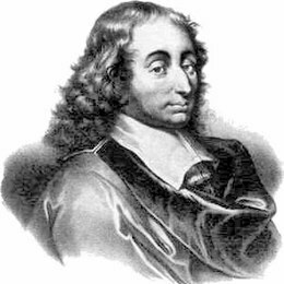 |  |  |
| (a) Blaise PASCAL | (b) Thomas BAYES | (c) Pierre-Simon LAPLACE |
| (1623–1662) | (1702–1761) | (1749–1827) |
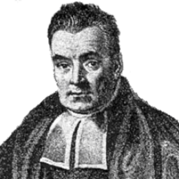
The discovery of Bayes. Thomas BAYES (cf. Fig. 5.12.b) was an XVIII English Presbyterian minister. Coming from a nonconformist family, he had read the work of Isaac NEWTON, David HUME and Abraham DE MOIVRE (McGrayne, 2011). His interest in game theory led him to imagine a thought experiment.
He derived Eq. () to solve this problem.
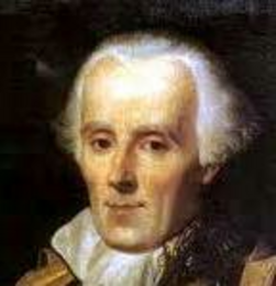
The contribution of Laplace. Pierre-Simon LAPLACE (cf. Fig. 5.12.c) was the son of a small estate owner, in Normandie. His father pushed him towards a religious career, that led him to study theology. He however quit at age 21 and moved to Paris, where he met the mathematician Jean LE ROND D’ALEMBERT, who helped him to get a teaching position. Laplace then had a successful scientific and political career (cf. Hahn, 2005, for a complete biography). Among his many other scientific contributions, Laplace is the true pioneer in the development of statistics using Bayes’ rule. Some authors even argue that we should call the approach presented in Sect. 5.1 “Bayesian-Laplacian” rather than simply “Bayesian”. After having read the memoir of Abraham DE MOIVRE, he indeed understood that probabilities could be used to quantify experimental uncertainties. His 1774 memoir on “the probability of causes by events” (Laplace, 1774) contains the first practical application of Bayes’ rule. His rule of succession, giving the probability of an event knowing how many times it happened previously, was applied to give the probability that the Sun will rise again. Laplace rediscovered Bayes’ rule. He was only introduced to Bayes’ essay in 1781, when Richard PRICE came to Paris. Laplace had a Bayesian conception of probabilities: “in substance, probability theory is only common sense reduced to calculation; it makes appreciate with accuracy what just minds can feel by some sort of instinct, without realizing it” (Laplace, 1812).
The rejection of Laplace’s work. The frequentist movement was initiated by British economist John Stuart MILL, only ten years after the death of Laplace. There were several reasons for this reaction (Loredo, 1990; McGrayne, 2011).
Mill’s disdain for the Bayesian approach was unhinged: “a very slight improvement in the data, by better observations, or by taking into fuller consideration the special circumstances of the case, is of more use than the most elaborate application of the calculus of probabilities founded on the data in their previous state of inferiority. The neglect of this obvious reflection has given rise to misapplications of the calculus of probabilities which have made it the real opprobrium of mathematics.” (Mill, 1843). The early anti-Bayesian movement was led by English statistician Karl PEARSON (cf. Fig. 5.13.a). Pearson developed: (i) the chi-squared test; (ii) the standard-deviation; (iii) the correlation coefficient; (iv) the -value; (v) the Principal Component Analysis (PCA). His book, “The Grammar of Science” (Pearson, 1892), was very influential, in particular to the young Albert EINSTEIN. Despite these great contributions, Pearson was a social Darwinist and a eugenicist.
 |  |  |
| (a) Karl PEARSON | (b) Ronald FISHER | (c) Jerzy NEYMAN |
| (1857–1936) | (1890–1962) | (1894–1981) |
The golden age of frequentism (1920-1930). Ronald FISHER (cf. Fig. 5.13.b) followed the way opened by Pearson. He is the most famous representative of the frequentist movement. He developed: (i) the maximum likelihood; (ii) NHST; (iii) the F-distribution and the F-test. His 1925 book, “Statistical Methods for Research Workers” (Fisher, 1925), was widely used in academia and industry. Despite the criticism we can address to the frequentist approach, Fisher’s contributions gave guidelines to rigorously interpret experimental data, that brought consistency to science. Fisher, who was like Pearson a eugenicist, was also paid as a consultant by the “Tobacco Manufacturer’s Standing Committee”. He spoke publicly against a 1950 study showing that tobacco causes lung cancer, by resorting to “correlation does not imply causation” (Fisher, 1957). Besides Pearson and Fisher, Jerzy NEYMAN (cf. Fig. 5.13.c) was also a prominent figure of frequentism at this time. These scientists, also known for their irascibility, made sure that nobody revived the methods of Laplace. McGrayne (2011) estimates that this golden era culminated in the 1920s-1930s.
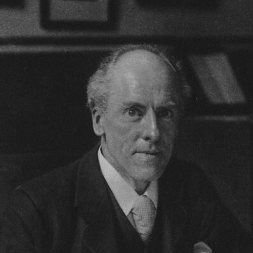
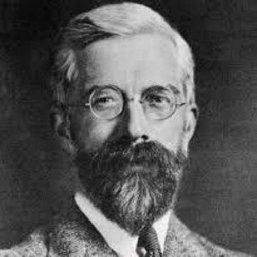
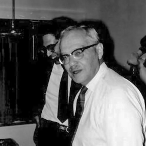
The Bayesian resistance. Several prominent scientists, who were not intimidated by Fisher and his colleagues, perpetuated the Bayesian approach (McGrayne, 2011). Among them, we can cite the following two.
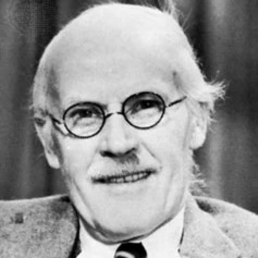 | 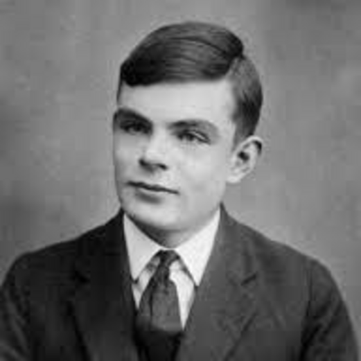 |  |
| (a) Harold JEFFREYS | (b) Alan TURING | (c) Edwin T. JAYNES |
| (1891–1989) | (1912–1954) | (1922–1998) |
After World War II. The first computers were built during the war. Bayesian techniques were now becoming feasible. Their use rapidly increased in the early 1950s. McGrayne (2011) note a few of them.
The great numerical leap forward. In the 1970s, the increasing power of computers opened new horizons to the Bayesian approach. The Metropolis-Hastings algorithm (cf. Sect. 5.1.3; Hastings, 1970) provided a fast, easy-to-implement method, which rendered Bayesian techniques more attractive. Gibbs sampling (cf. Sect. 5.1.3; Geman & Geman, 1984), which can be used to solve complex problems, put Bayes’ rule into the spotlight. We can note the following achievements.
At the same time, Edwin JAYNES (cf. Fig. 5.14.c) was working at solidifying the mathematical foundations of the Bayesian approach. It culminated in his posthumous book, “Probability Theory: The Logic of Science” (Jaynes, 2003).
Bayesian techniques, nowadays. Looking at the contemporary literature, it appears that Bayesians have won over frequentists 9. In a lot of cases, this is however only a fashion trend due to the fact that the word “Bayesian” became hip in the 2010s, in astrophysics. There are already misuses of Bayesian methods. This is unavoidable. This might result from the fact that there is still a generation of math teachers and the majority of statistical textbooks ignoring the Bayesian approach. The difference with -hacking is that Bayesian-hacking is easier to spot, because interpreting posterior distributions is less ambiguous than NHST. The supremacy of Bayesian techniques is ultimately demonstrated by the success of Machine-Learning (ML). ML has Bayesian foundations. It is a collection of probabilistic methods. Using ML can be seen as performing posterior inference, based on the evidence gathered during the training of the neural network.
The following epistemological considerations have been expressed in several texts (e.g. Good, 1975; Loredo, 1990; Jaynes, 2003; Hoang, 2020). The book of Jaynes (2003) is probably the most rigorous on the subject, while the book of Hoang (2020) provides an accessible overview.
Epistemology treats several aspects of the development of scientific theories, from their imagination to their validation. We will not discuss here how scientists can come up with ground-breaking ideas. We will only focus on how a scientific theory can be experimentally validated.
Scientific positivism. The epistemological point of view of Auguste COMTE (cf. Fig. 5.15.a) had a considerable influence on the XIX century epistemology, until the beginning of the XX century. Comte was a French philosopher and sociologist, who developed a complex classification of sciences and theorized their role in society. What is interesting for the rest of our discussion is that he was aiming at demarcating sciences from theology and metaphysics. He proposed that we need to renounce to understand the absolute causes (why), to focus on the mathematical laws of nature (how). In that sense, his system, called positivism, is not an empiricism (e.g. Grange, 2002). Comte stressed that a theoretical framework is always necessary to interpret together different experimental facts. His approach is a reconciliation of empiricism and idealism, where both viewpoints are necessary to make scientific discoveries. Positivism is not scientism, either. Comte’s view was, in substance, that science provides a knowledge that is rigorous and certain, but at the same time only partial and relative.
 |  |  |
| (a) Auguste COMTE | (b) Henri POINCARÉ | (c) Karl POPPER |
| (1798–1857) | (1854–1912) | (1902–1994) |
Conventionalism and verificationism. At the beginning of the XX century, two complementary epistemological points of view were debated.
We now review the epistemology developed by Karl POPPER (cf. Fig. 5.15.c), which is the center of our discussion. Popper was an Austrian-born British philosopher who had a significant impact on the modern scientific method 10. His concepts of falsifiability and reproducibility are still considered as the standards of the scientific method, nowadays. His major book, “The Logic of Scientific Discovery” (Popper, 1959), was originally published in German in 1934, and rewritten in English in 1959. Before starting, it is important to make the distinction between the following two terms.
The criticism of induction. Popper’s reflection focusses on the methods of empirical sciences. The foundation of his theory is the rejection of inductive logic, as he deems that it does not provide a suitable criterion of demarcation, that is a criterion to distinguish empirical sciences from mathematics, logic and metaphysics. According to him, the conventionalist and verificationist approaches are not rigorous enough. Popper argues that only a deductivist approach provides a reliable empirical method: “hypotheses can only be empirically tested and only after they have been advanced” (Popper, 1959, Sect. I.1). Deductivism is however not sufficient in Popper’s mind.
Falsifiability. Popper criticizes conventionalists who “evade falsification by using ad hoc modifications of the theory”. For that reason, verifiability is not enough. Empirical theories must be falsifiable, that is they must predict experimental facts that, if empirically refuted, will prove them wrong. His system, which was afterward called falsifiabilism, is the combination of: (i) deductivism; and (ii) modus tollens. The modus tollens is the following logical proposition:
| (5.37) |
Put in words, it can be interpreted as: if a theory T predicts an observational fact D, and this fact D happens to be wrong, then we can deduce that the theory T is wrong. This principle is to be strictly applied: “one must not save from falsification a theory if it has failed” (Popper, 1959, Sect. II.4). Let’s take a pseudo-science example to illustrate Popper’s point. Let’s assume that a “ghost expert” pretends a ghost inhabits a given haunted house. The verificationist approach would consist in saying that, to determine if there is really a ghost, we need to go there and see if it shows up. Popper would argue that, if the ghost did not appear, our expert would claim that it was because it was intimidated or it felt our skepticism. Falsifiabilism would dictate to set experimental conditions beforehand by agreeing with the expert: if the ghost does not appear in visible light, in this house, at midnight, on a particular day, then we will deduce that this ghost theory is wrong. The ghost expert would probably not agree with such strict requirements. Popper would thus conclude that ghostology is not an empirical science.
Reproducibility. A difficulty of the empirical method is relating perceptual experiences to concepts. Popper argues that the objectivity of scientific statements lies in the fact that they can be inter-subjectively tested. In other words, if several people, with their own subjectivity, can perform the same empirical tests, they will rationally come to the same conclusion. This requires reproducibility. Only repeatable experiments can be tested by anyone. Reproducibility is also instrumental in avoiding coincidences.
Parsimony (Ockham’s razor). A fundamental requirement of scientific theories is that they should be the simplest possible. Unnecessarily complex theories should be eliminated. This is the principle of parsimony. Popper is aware of that and includes it in his system. This is however not the most convincing point of his epistemology. His idea is that a simple theory is a theory that has a high degree of falsifiability, which he calls “empirical content” (Popper, 1959, Sect. II.5). In other words, according to him, the simplest theories are those that have the highest prior improbability, whereas complex theories tend to have special conditions that help them evade falsification.
Popper’s epistemology is frequentist. It is obvious that Popper’s system has a frequentist frame of mind. It was indeed conceived at the golden age of frequentism (cf. Sect. 5.2.1.2).
We now discuss how the Bayesian approach provides an alternative to Popper’s epistemology. Jaynes (2003) demonstrates that probabilities, in the Bayesian sense, could be the foundation of a rigorous scientific method. Hoang (2020) even argues that Bayes’ rule is the optimal way to account for experimental data.
Falsifiability and the limits of Platonic logic. The refusal of Popper and frequentists to adopt probabilistic logic is the reason why their decision upon experimental evidence is so convoluted. The application of Platonic logic to the physical reality indeed presents some issues. One of the most famous aporias is “Hempel’s paradox” (Hempel, 1945). It states the following.
| (5.38) |
The example taken by Hempel (1945), is “all ravens are black” (). The contraposition is “anything that is not black is not a raven” (). From an experimental point of view, if we want to corroborate that all ravens are black, we can either: (i) find black ravens (i.e. verifying the proposition); or (ii) find anything that is neither black nor a raven, such as a red apple (i.e. verifying the contraposition). The second solution is obviously useless in practice. To take an astrophysical example, finding a quiescent H I cloud would be considered as a confirmation that star formation occurs only in H2 clouds. This is one of the reasons why Popper requires falsifiability.
| (5.39) |
The difference is that, with probabilities, we can deal with uncertainty, that is . Second, Bayes factors quantify the strength of evidence (cf. Sect. 5.1.4.1), and it is different in the case of a black raven or a red apple. Good (1960) shows that the strength of evidence is negligible in the case of a red apple. The Bayesian solution is thus the most sensible one. Bayes factors are therefore the tool needed to avoid requiring falsifiability. We can adopt a verificationist approach and discuss if our data brought significant evidence.
Bayesianism does not require falsifiability. Bayes factors provide a way to quantify the strength of evidence brought by any data set.
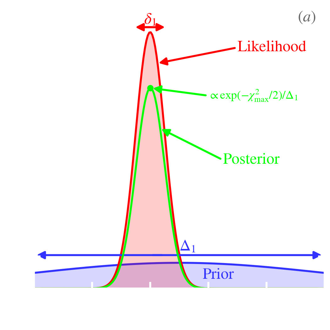
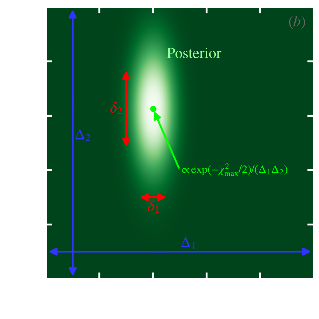
Parsimony is hard-coded in Bayes’ rule. The principle of parsimony is directly implied by the use of Bayes factors. To illustrate this point, let’s assume we are fitting a two-parameter model to a data set, , and we want to know if we can fix the second parameter (model ) or let it free (model ). The Bayes factor (Eq. ) is simply:
| (5.40) |
Let’s assume that we have a Gaussian model. We can write the product of the prior and the likelihood, in this case:
| (5.41) |
where we have assumed that the prior was flat over and that we had observations with uncertainty . Notice that the product in Eq. () is proportional but not equal to the posterior. We indeed have not divided it by , as this is the quantity we want to determine. If we approximate the posterior by a rectangle, we obtain the following rough expression, using the notations in Fig. 5.16.a:
| (5.42) |
Let’s assume that adding parameter does not improve the fit. The thus stays the same. This is represented in Fig. 5.16.b. With the same assumptions as in Eq. (), we obtain:
| (5.43) |
Eq. () thus becomes:
| (5.44) |
It thus tell us that model is more credible. The penalty of adding the extra parameter is . More generally, we can encounter the three following situations.
 |  |
Comparison of the Bayesian and Popperian methods. We can now compare both approaches. The following arguments are summarized in Table 5.3.
| (5.45) |
| Bayesian | Popperian |
|
| Corroboration | Verifiability & strength of evidence | Requires falsifiability |
| Logic | Probabilistic: continuity between skepticism & confidence | Platonic: theories are either true or false at a given time |
| Repeatability | Can account for unique data | Requires reproducibility |
| Experimental data | Can account for small, heterogeneous data sets | Experimental settings need to be defined beforehand |
| External data | Holistic approach | No possibility to account for any data outside of the experiment |
| Parsimony | Bayes factors eliminate unnecessary complex theories | The most falsifiable theories are preferred |
| Knowledge growth | Prior accounts for past knowledge | Each experiment is independent |
| Attitude | Universal approach: can test any theory | Partial approach: only one theory can be tested |
| Application | Most scientists are unconsciously pragmatic Bayesians | Strict Popperians are rare & probably not very successful |
We now demonstrate what the Bayesian methods, which constitute a true epistemological approach, can bring to ISD studies. In particular, we advocate that hierarchical Bayesian models are an even better application of this approach. We illustrate this point with our own codes.
We have discussed throughout this manuscript the difficulty to constrain dust properties using a variety of observational constraints. For instance, we have seen that there is a degeneracy between small and hot equilibrium grains in the MIR (cf. Sect. 3.1.2.2), or between the effects of the size and charge of small a-C(:H) (cf. Sect. 3.2.1.3). In a sense, we are facing what mathematicians call an ill-posed problem, with the difference that we do not have the luxury of rewriting our equations, because they are determined by the observables. We detail these issues below.
Degeneracy between microscopic and macroscopic properties. When we observe a [C II] line, we know it comes from a C atom, and we can characterize very precisely the physical nature of this atom. On the contrary, if we observe thermal grain emission, we know it can come from a vast diversity of solids, with different sizes, shapes, structures, and composition. Even if we observe a feature, such as the 9.8 silicate band or an aromatic feature, we still have a lot of uncertainty about the physical nature of its carrier. This is the fundamental difference between ISM gas and dust physics. The complexity of gas modeling comes from the difficulty to determine the variation of the environmental conditions within the telescope beam. This difficulty thus comes from our uncertainty about the macroscopic distribution of ISM matter and of the energy sources (stars, AGNs, etc.) in galaxies. We also have the same issue with dust. When studying ISD, we therefore constantly face uncertainties about both the microscopic and macroscopic properties. Assuming we have a model that accounts for variations of both the dust constitution and the spatial distribution of grains relative to the stars, the Bayesian approach is the only way to consistently explore the credible regions of the parameter space, especially if several quantities are degenerate. We will give some examples in Sect. 5.3.3.
Heterogeneity of the empirical constraints. A dust model, such as those discussed in Sect. 2.3, has been constrained from a variety of observables (cf. Sect. 2.2): (i) from different physical processes, over the whole electromagnetic spectrum; (ii) originating from different regions in the MW; (iii) with prior assumptions coming from studies of laboratory analogues and meteorites. When we use such a model to interpret a set of observations, we should in principle account for all the uncertainties that went into using these constraints:
Obviously, only the Bayesian approach can account for these, especially knowing that these different uncertainties will likely be non-Gaussian and partially correlated. This is however an ambitious task, and it has been done only approximately (e.g. Sect. 4.1.3 of Galliano et al., 2021). This is a direction that future dust studies should take.
The observables are weakly informative. Another issue with ISD studies is that the observables, taken individually, bring a low weight of evidence. A single broadband flux is virtually useless, but a few fluxes, strategically distributed over the FIR SED, can unlock the dust mass and starlight intensity (cf. Sect. 3.1.2.2). Yet, these different fluxes come from different observation campaigns, with different instruments. If we add that the partially-correlated calibration uncertainties of the different instruments often dominate the error budget, we understand that the Bayesian approach is the only one that can rigorously succeed in this type of analysis. We will discuss the treatment of calibration uncertainties in Sect. 5.3.2.2.
Contaminations are challenging to subtract. The different sources of foreground and background contaminations, that we have discussed in Sect. 3.1.3.2, will become more and more problematic with the increasing sensitivity of detectors. Indeed, probing the diffuse ISM of galaxies requires to observe surface brightnesses similar to the MW foreground. In addition, the CIB is even brighter at submm wavelengths (cf. Fig. 3.24). These two contaminations, the MW and the CIB, have very similar SEDs and a complex, diffuse spatial structure. Accurately separating these different layers therefore requires probabilistic methods, using redundancy on large-scales (e.g. Planck Collaboration et al., 2016a). It requires modeling every component at once. Bayesian and ML methods are the most obvious solutions.
We now discuss the formalism of hierarchical Bayesian inference, applied to SED modeling. This method has been presented by Kelly et al. (2012) and Galliano (2018).
Posterior of a single source. Let’s assume that we are modeling a single observed SED (e.g. one pixel or one galaxy), sampled in broadband filters, that we have converted to monochromatic luminosities: (). Let’s assume that these observations are affected by normal iid noise, with standard-deviation . If we have a SED model, depending on a set of parameters , such that the predicted monochromatic luminosities in the observed bands is , we can write that:
| (5.46) |
where . In other words, our observations are the model fluxes plus some random fluctuations distributed with the properties of the noise. The distribution of the parameters, , is what we are looking for. We can rearrange Eq. () to isolate the random variable:
| (5.47) |
Since we have assumed iid noise, the likelihood of the model is the product of the likelihoods of each individual broadbands:
| (5.48) |
were . If we assume a flat prior, the posterior is (Eq. ):
| (5.49) |
The difference is that: (i) in Eq. (), the parameters, , are assumed fixed, the different are thus independent; whereas (ii) in Eq. (), the observations, , are assumed fixed, the different terms in the product are now correlated, because each depends on all the parameters.
Modeling several sources together. If we now model sources with observed luminosities, (), to infer a set of parameters, , the posterior of the source sample will be:
| (5.50) |
Notice that, in the second equality, the different are independent, as each one depends on a distinct set of parameters, . The sampling of the whole posterior distribution will thus be rigorously equivalent to sampling each individual SED, one by one.
With a non-hierarchical Bayesian approach, the sources in a sample are independently modeled.
Nuisance variables are parameters we need to estimate to properly compare our model to our observations. The particular value of these variables is however not physically meaningful, and we end up marginalizing the posterior over them. The Bayesian framework is particularly well-suited for the treatment of nuisance parameters.
Calibration uncertainties. Calibration errors originate from the uncertainty on the conversion of detector readings to astrophysical flux (typically ADU/s to Jy/pixel). Detectors are calibrated by observing a set of calibrators, that are bright sources with well-known fluxes. The uncertainties in the observations of these calibrators and on the true flux of the calibrators translate into a calibration uncertainty.
Introduction into the posterior. To account for calibration uncertainties, we can rewrite Eq. () as:
| (5.51) |
We have now multiplied the model by , where is a random variable following a centered multivariate normal law 15 with covariance matrix, . This random variable, which represents a correction to the calibration factor, is multiplicative: it scales the flux up and down. contains all the partial correlations between wavelengths (cf. Appendix A of Galliano et al., 2021). The important point to notice is that the do not depend on the individual object (index ), they are unique for the whole source sample. The posterior of Eq. () now becomes:
| (5.52) |
where is the prior on . We can make the following remarks.
The posterior of the parameters is, in the end, the marginalization over of Eq. ():
| (5.53) |
Calibration errors can be rigorously taken into account as nuisance parameters.
Accounting for the evidence brought by each source. In Sect. 5.1.2.2, we have stressed that, when performing a sequential series of measure, we can use the previous posterior as the new prior. Yet, the posterior in Eq. () does not allow us to do so, as: (i) the posteriors of individual sources all depend on , they must therefore be sampled at once; and (ii) the parameters, , are not identical, we are not repeating the same measure several times as in Eq. (), we are observing different sources. Accounting for the accumulation of evidence is thus not as straightforward as in Eq. (). There is however a way to use an informative prior, consistently constrained by the sample. It is the Hierarchical Bayesian (HB) approach. To solve the conundrum that we have just exposed, we can make the following assumptions.
The hierarchical posterior. With the HB approach, the full posterior of our source sample is:
| (5.54) |
| (5.55) |
For the composite model (; cf. Sect. 3.1.2.2), constrained by wavelengths, and for sources or pixels, we would have to sample a dimension parameter space.
We now present practical illustrations of SED modeling with the HB approach. The first HB dust SED model was presented by Kelly et al. (2012). It was restrained to single MBB fits. Veneziani et al. (2013) then presented a HB model that could be applied to a combination of MBBs. The HiERarchical Bayesian Inference for dust Emission code (HerBIE; Galliano, 2018), was the first HB model, and to this day the only one to our knowledge, to properly account for full dust models, with: (i) realistic optical properties; (ii) complex size distributions; (iii) rigorous stochastic heating; (iv) mixing of physical conditions; (v) photometric filter and color corrections; and (vi) partially-correlated calibration errors. The following examples have been computed with HerBIE.
To demonstrate the efficiency of the HB method and the fact that it performs better than its alternatives, we rely on the simulations presented by Galliano (2018). These simulations are simply obtained by randomly drawing SED model parameters from a multivariate distribution, for a sample of sources. This distribution is designed to mimic what we observe in typical star-forming galaxies. The SED model used is the composite approach (cf. Sect. 3.1.2.2), except when we discuss MBBs. Each set of parameters result in an observed SED, that we integrate into the four IRAC, the three PACS and the three SPIRE bands. We add noise and calibration errors. This way we can test fitting methods and assess their efficiency by comparing the inferred and the true values.
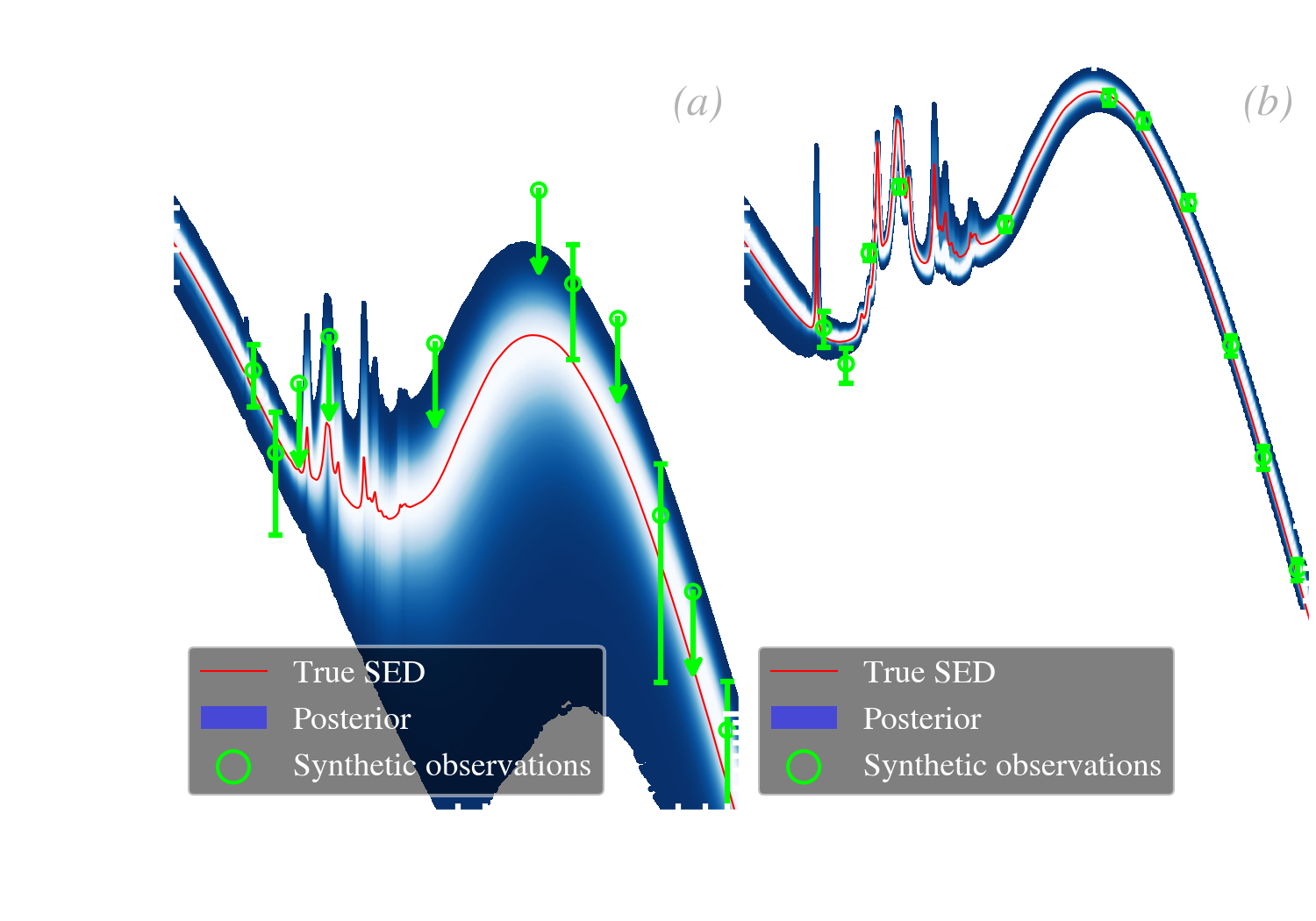
Close look at a fit. Fig. 5.19.a-b shows the posterior SED PDF of the faintest and brightest pixels in a simulation, fitted in a HB fashion.
In a HB model, the least-constrained sources are more corrected by the prior than the brightest ones.
 | 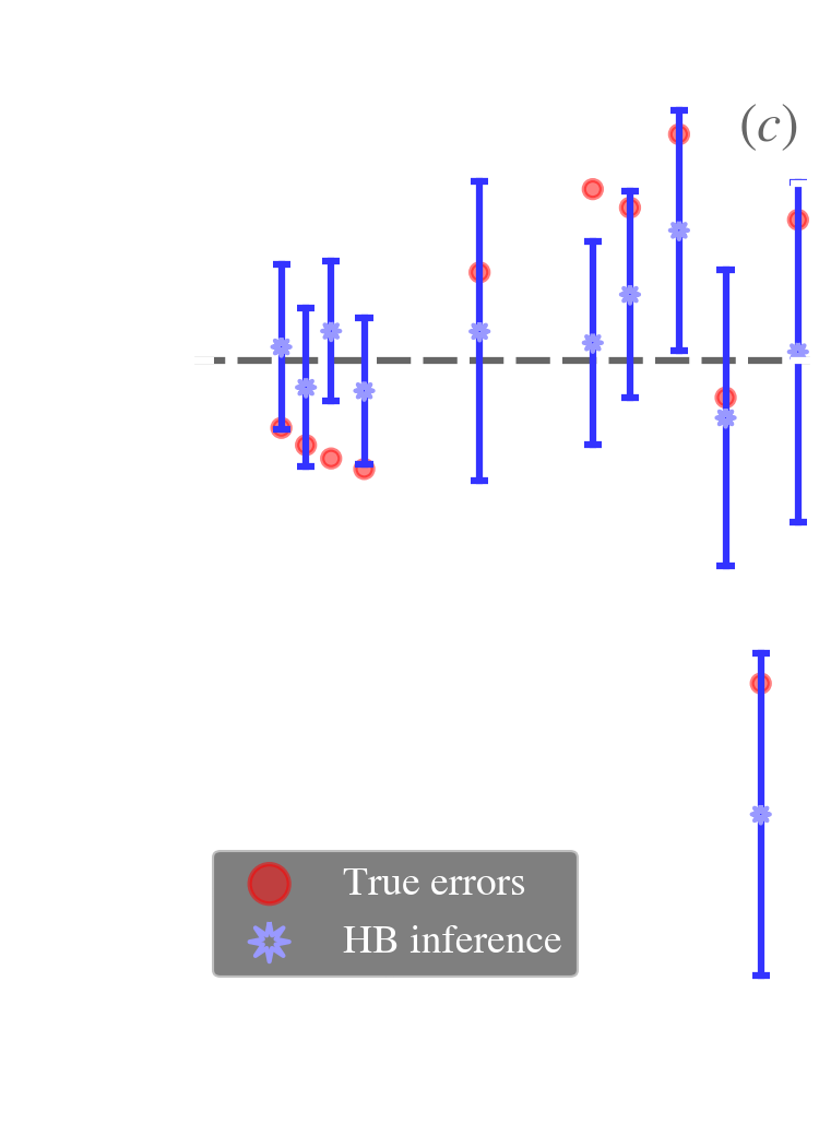 |
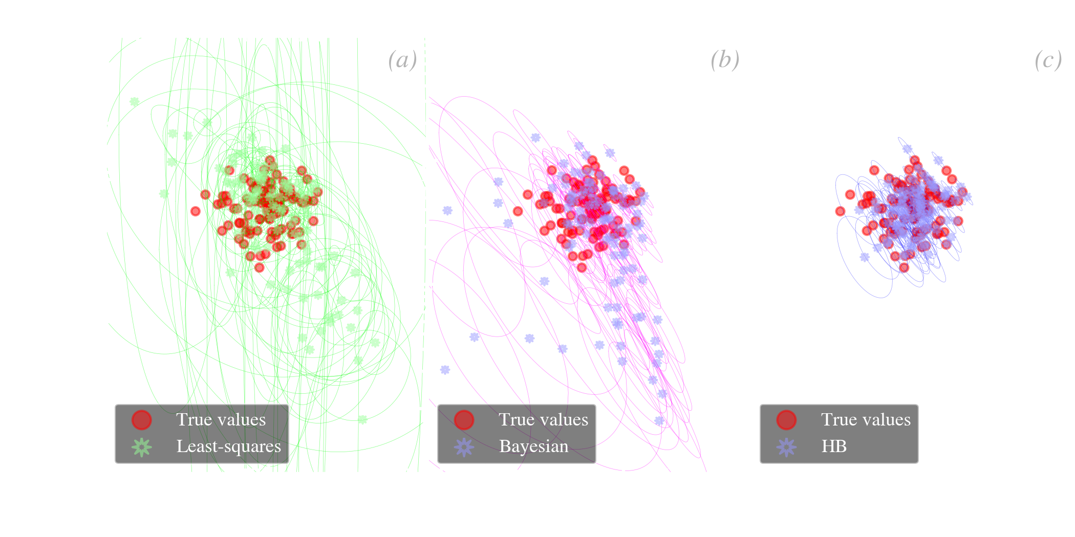
Comparison between different approaches. We have been discussing the two extreme pixels of our simulation. Let’s now look at the whole source sample and compare several methods. Fig. 5.19 shows the same parameter space as in Fig. 5.18, but for all sources, with different methods.
This false correlation is typical of frequentist methods, but not exclusive. It is the equivalent of the degeneracy we have already discussed in Sect. 3.1.2.1. Because of the way the model is parametrized, if we slightly overestimate the dust mass, we will indeed need to compensate by decreasing , to account for the same observed fluxes, and vice versa. This false correlation is thus induced by the noise.
From a general point view, a HB method is efficient at removing the scatter between sources that is due to the noise. In addition, the inferred uncertainties on the parameter of a source are never larger than the intrinsic scatter of the sample, because this scatter is also the width of the prior. For instance, in Fig. 5.19.c, the lowest signal-to-noise sources (lower left side of the distribution) have uncertainties (blue ellipses) similar to the scatter of the true values (red points), because the width of the prior matches closely this distribution. On the opposite, the uncertainties of high signal-to-noise sources (upper right side) are much smaller, they are thus not significantly affected by the prior.
HB methods are efficient at recovering the true, intrinsic scatter of parameters and their correlations.
|
| HB | True |
|
|
| 0 |
|
|
| 0.5 |
|
|
| 3.742 |
|
|
| 0.4 |
|
|
| 0 |
|
|
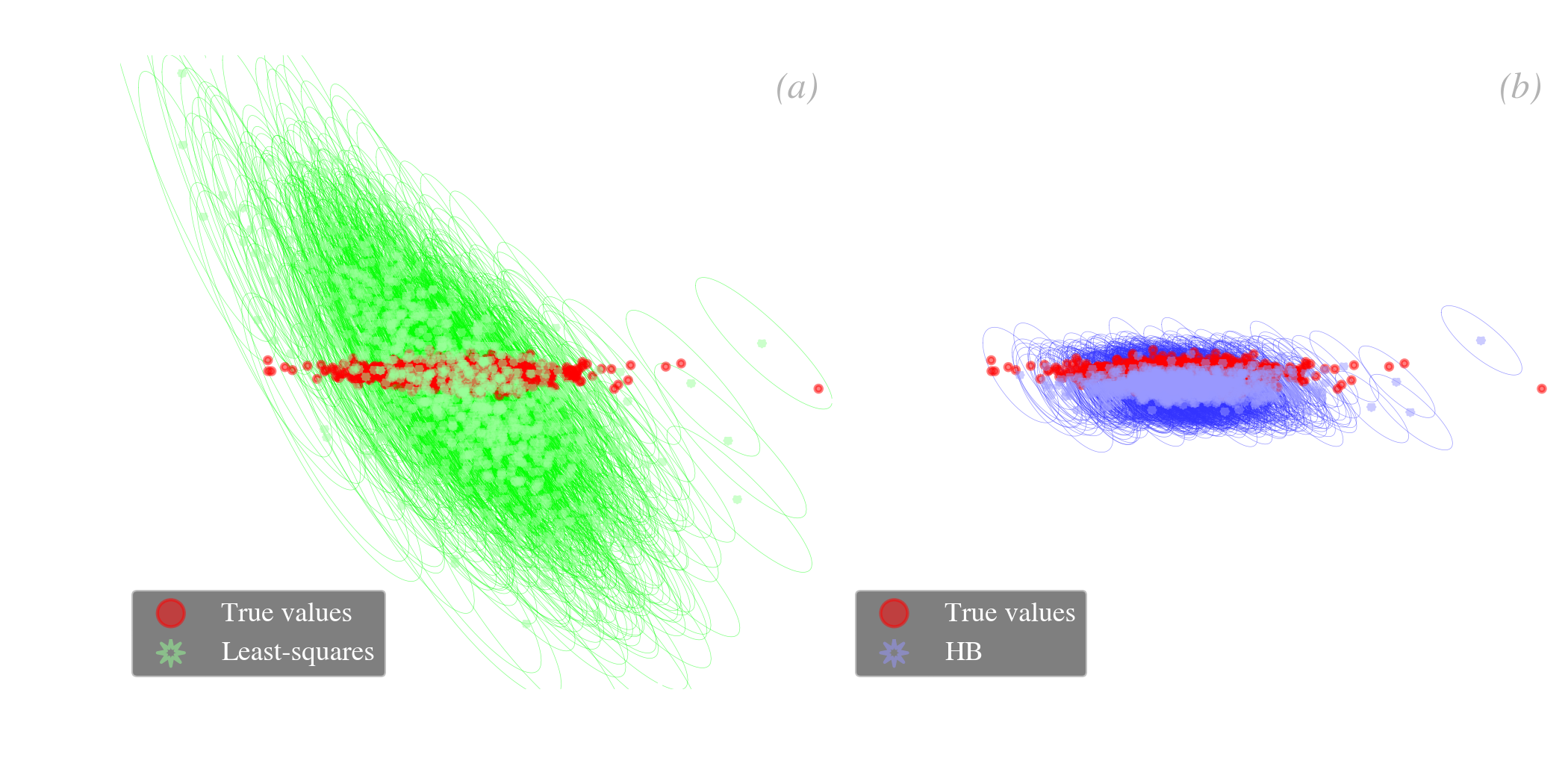
The emissivity-index-temperature degeneracy of MBBs. We have just seen that HB methods are efficient at removing false correlations between inferred properties. We emphasize that HB methods do not systematically erase correlations if there is a true one between the parameters (cf. the tests performed in Sect. 5.1 of Galliano, 2018, with intrinsic positive and negative correlations). This potential can obviously be applied to the infamous correlation discussed in Sect. 3.1.2.1. This false correlation has been amply discussed by Shetty et al. (2009). Kelly et al. (2012) showed, for the first time, that HB methods could be used to solve the degeneracy. Fig. 5.20 shows the results of Galliano (2018) on that matter. We can see that the false negative correlation obtained with a least-squares fit (Fig. 5.20.a) is completely eliminated with a HB method (Fig. 5.20.b).
We now further develop and illustrate the instrumental role of the hierarchical prior.
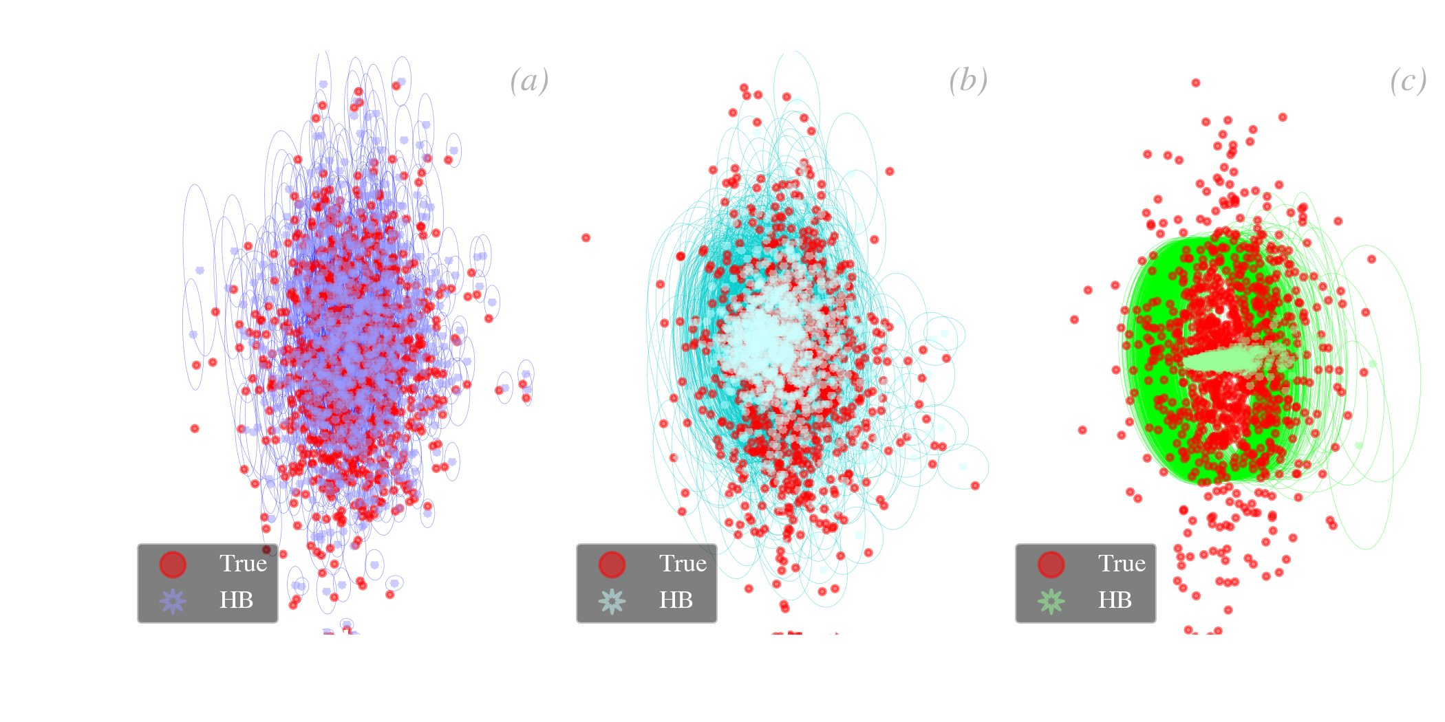
Linking the different sources. We have noted in Eq. () that the hierarchical prior was breaking the independency between the different sources in the sample, encountered in the non-hierarchical Bayesian case. This is because the properties of the prior (the hyperparameters) are inferred from the source distribution, and the properties of the individual sources are affected, in return, by this prior. This is illustrated in Fig. 5.21. This figure shows the HB fits of three simulations, varying the median signal-to-noise ratio of the sample. We have represented a different parameter space, this time.
HB methods are useful when the parameter uncertainty of some sources is comparable to or larger than the scatter of this property over the whole sample.
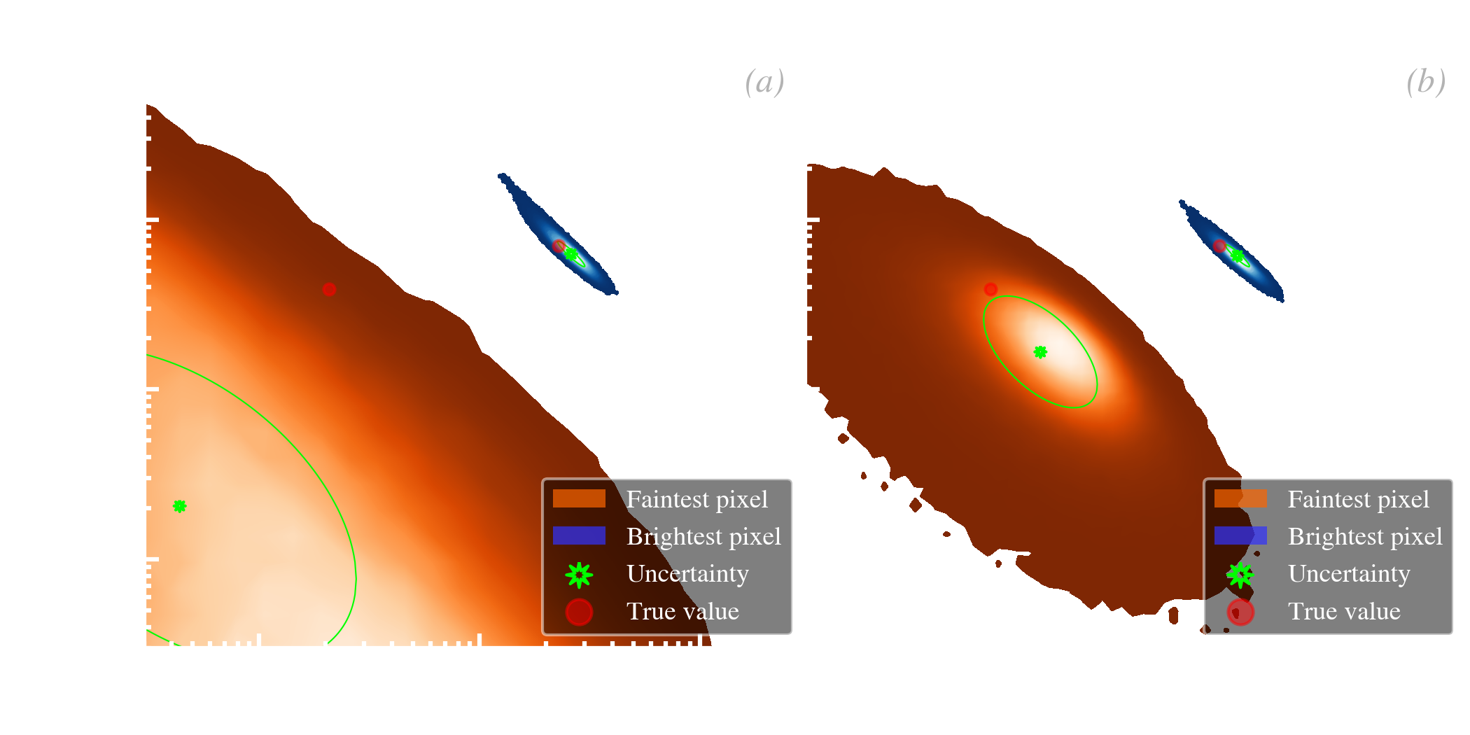
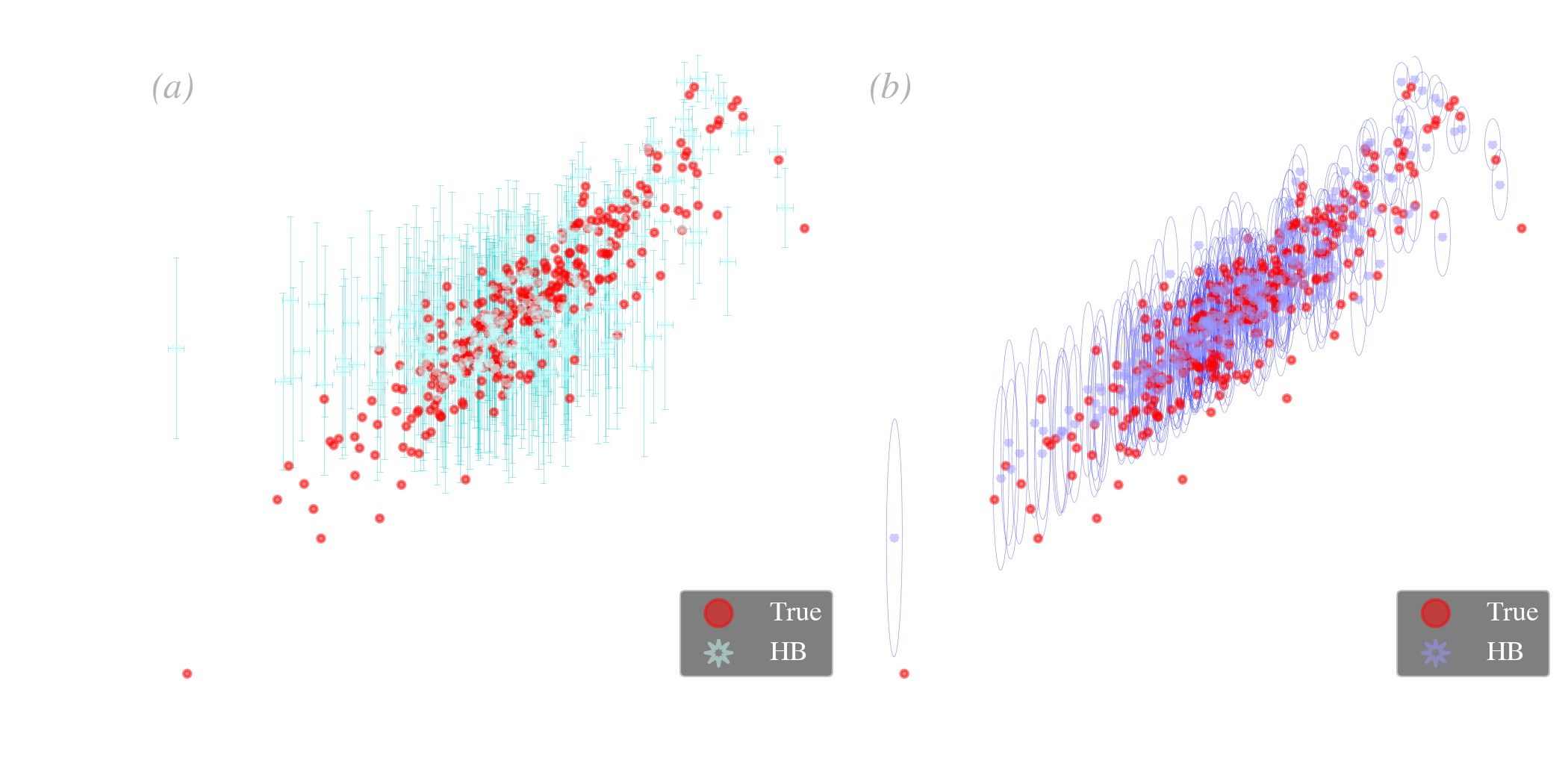
Holistic prior. From a statistical point of view, it is always preferable to treat all the variables we are interested in as if they were drawn from the same multivariate distribution, however complex it might be. Stein (1956) showed that the usual estimator of the mean () of a multivariate normal variable is inadmissible (for more than two variables), that is we could always find a more accurate one. In other words, if we were interested in analyzing together several variables, not necessarily correlated, such as the dust and stellar masses, it would always be more suitable to use estimators that combine all of them. This is known as Stein’s paradox. Although Stein (1956)’s approach was frequentist, this is a general conclusion. From a Bayesian point of view, it means that we should put all the variables we are interested in analyzing, even if they are not SED model parameters, in the prior. In addition, if these external variables happen to be correlated with some SED model parameters, they will help refining their estimates. This is illustrated in Fig. 5.22. We show in both panels a simulation of the correlation between the dust mass, which is a SED model parameter, and the gas, which is not. When performing a regular HB fit, and plotting the correlation as a function of , we obtain the correlation in Fig. 5.22.a. We see that the agreement with the true values breaks off at low mass (also the lowest signal-to-noise). If we now include in the prior 16, we obtain the correlation in Fig. 5.22.b. It provides a much better agreement with the true values. This is because adding in the prior brought some extra information. The information provided by a non-dusty parameter helped refine the dust SED fit. For instance, imagine that you have no constraints on the dust mass of a source, but you know its gas mass. You could infer its dust mass by taking the mean dustiness of the rest of the sample. This holistic prior does that, in a smarter way, as it accounts for all the correlations in a statistically consistent way.
The HB approach allows an optimal, holistic treatment of all the quantities of interest, even if they are not related to the dust.
SED modeling is far from the only possible application of HB methods. We briefly discuss below two other models we have developed.
Cosmic dust evolution. The dust evolution model we have discussed in Sect. 4.3 has been fitted to galaxies by Galliano et al. (2021), in a HB way. To be precise, we have used the output of HerBIE, , , , SFR and metallicity, as observables. We then have modeled the SFH-related parameters in a HB way, and have assumed that the dust efficiencies were common to all galaxies (i.e. we inferred one single value for the whole sample). These common parameters were not in the hierarchical prior, because their value is the same for all galaxies. They were however sampled with the other parameters, in a consistent way. We were successful at recovering dust evolution timescales consistent with the MW at Solar metallicity (cf. Sect. 4.3.1.2). One important improvement would be to treat everything within the same HB model: (i) the SED; (ii) the stellar and gas parameters; and (iii) the dust evolution. This is something we plan to achieve in the near future.
MIR spectral decomposition. The type of MIR spectral decomposition that we have discussed in Sect. 3.2.1.2 could also benefit from the HB approach. Although the model is mostly linear, there are a lot of degeneracies between the uncertainties of adjacent blended bands, such as the 7.6 and 7.8 features. In addition, plateaus and weak features are usually poorly constrained and their intensity can considerably bias the fit at low signal-to-noise. Hu et al. (in prep.) have developed such a HB MIR spectral decomposition tool. Its efficiency has been assessed on simulated data, and it is now being applied to M 82. This model will be valuable to analyze the spectra from the JWST.
1.Epistemology is the philosophical study of the nature, origin and limits of human knowledge. By extension, it is the philosophy of science.
2.It is often considered as the scientific definition of probabilities, while we will show later that the Bayesian definition has more practical applications.
3.Our variable is the true flux. It is positive. Measured fluxes can occasionally be negative because of noise fluctuations.
4.The distribution in Fig. 5.5.a has a very narrow tail on the lower side of . It can thus in principle be lower, but this is such a low probability event that, for the clarity of the discussion, we will assume this is unlikely.
5.Numerous authors publish articles claiming to have solved a problem using “MCMC methods”. This is not the best terminology to our mind, especially knowing that MCMCs can be used to sample any distribution, not only a Bayesian posterior. These authors should state instead to have solved a problem in a Bayesian way (what), using a MCMC numerical method (how). The same way, we tell our students to say that they “modeled the photoionization”, rather than they “used Cloudy”.
6.This quantity is problematic to compute. Sokal (1996) and Foreman-Mackey et al. (2013) discuss an algorithm to evaluate it numerically.
7.The acceptance of a wrong hypothesis (false positive) is called “type I error”, whereas the rejection of a correct hypothesis (false negative) is called “type II error”.
8.Pascal’s wager states that it is rational to act as if God existed. If God indeed exists, we will be rewarded, which is a big win. If He doesn’t, we will have only renounced to some material pleasures, which is not a dramatic loss.
9.There are still a few frequentist trolls roaming Wikipedia’s mathematical pages.
10.If journalists are reading these lines, we stress that the peer-review process has nothing to do with the scientific method. It is just a convenient editorial procedure that filters poorly thought-out studies.
11.This could be called “P(opper)-hacking”.
12.Nowadays, scientists call “reproducibility” the action of providing the data and the codes a publication was prepared with. This is a good practice, but this is not Popper’s reproducibility. It should rather be qualified as “open source”.
13.Concerning the topics discussed in Sect. 4.3, we have seen this attitude in a small group of people trying to prove ISM dust is stardust, constantly ignoring the big picture summarized in Table 4.2.
14.In this example, is not the calibration uncertainty, but the error made because of the calibration uncertainty.
15.We could have taken a different distribution, such as a Student’s (e.g. Eq. 31 of Galliano, 2018).
16.From a technical point of view, including an external parameter in the prior, such as , can be seen as adding an identity model component: . Concretely, it means that, at each iteration, we sample from its uncertainty distribution, and the distribution of and its potential correlations with the other parameters inform the prior.
_-_Gu%C3%A9rin.jpg)