
This is not a new result – Draine & Salpeter (1979) reached the
conclusion that grain destruction was rapid and that regrowth of dust
in the ISM was required to explain the observed depletions. The
numbers basically haven’t changed appreciably since then; the argument
has been reiterated a number of times (...). Nevertheless, some authors
continued to hold the view that the solids in the interstellar medium
were primarily formed in stars.
(Bruce T. DRAINE; Draine, 2009)
This chapter focusses on the study of dust evolution in all interstellar environments, at all spatial scales. Dust evolution is the variation of the constitution of a grain mixture with time, under the effects of its environment. The timescales of evolution being significantly longer than the career of a scientist, we usually study spatial variations of the dust content in a region, or the variations among a sample of galaxies. These different observations are then compared, being considered as snapshots at different evolutionary stages. The environmental parameters that are commonly used to quantify dust evolution are: (i) the ISM density and the ISRF intensity and hardness, for spatially-resolved studies; (ii) the metallicity and star formation rate, for global galactic studies. The main processes responsible for dust evolution are represented on Fig. 4.1.
Stars have a crucial impact on ISD: (i) they synthesize the heavy elements that constitute dust grains (Fig. 2.16); (ii) they also directly produce dust seeds in their ejecta; (iii) the shock waves of SNe erode and vaporize the grains; (iv) the radiative and mechanical feedback of massive stars carve the ISM and process the grains.
A star can be conceptualized as a sphere of gas in hydrostatic equilibrium, where the gravity is counterbalanced by the thermal pressure sustained by nuclear reactions in its core (e.g. Degl’Innocenti, 2016, for an introduction). The energy produced in the core is carried out through radiation, convection or conduction. The initial mass of a star, and in a lesser extent its initial metallicity, determine its future evolution.
The nuclear reactions in stellar interiors, on top of being the fuel of stars, lead to the production of heavy elements. A fraction of these freshly synthesized elements are injected back into the ISM, during the final stages of stellar evolution.
Nuclear binding energies. A fundamental quantity to determine the efficiency of nuclear reactions to sustain the thermal pressure within a star is the nuclear binding energy of an element of mass A (number of nucleons; cf. e.g. Chaps. 1-2 of Pagel, 1997, for a review). This quantity is represented in Fig. 4.2 for the most relevant nuclei. To have an exothermic reaction, that will be able to counterbalance gravity, one needs to synthesize elements of higher binding energies. The curve of Fig. 4.2 reaches a maximum around Fe.
Primordial nucleosynthesis. Before the first stars appeared, H and He, as well as elements up to Li, were synthesized during the first 15 minutes after the big bang (e.g. Pagel, 1997; Calura & Matteucci, 2004; Johnson, 2019). The temperature was at this time around K. This primordial nucleosynthesis was brief, as the Universe was expanding and cooling. It is estimated that after 20 minutes, the temperature was too low to synthesize new elements. The primordial abundances refer to the elements produced during these first minutes (cf. Eq. ):
| (4.1) |
Stellar nucleosynthesis. Once the temperature at the center of a collapsing protostar becomes high enough ( K), thermonuclear reactions 1 are initiated. Several chains and cycles of reactions occur in stars, at different stages. The most important ones are the following (e.g. Filippone, 1986; Pagel, 1997; Silva Aguirre, 2018).
H burning, which encompasses both the p-p chain and the CNO cycle, represents the longest phase in the lifetime of a star, whereas He burning lasts only of its existence.
Stars are born from the collapse of molecular clouds into protostars (e.g. Motte et al., 2018, for a review). Protostars accrete matter until their winds and radiation pressure stops this process, leading to a pre-main sequence star (pre-MS). Pre-MS stars exhibit violent winds and bipolar jets, clearing away the remaining molecular cocoon they were born in. They contract until the temperature in their core is high enough to initiate H fusion ( K). Below , we get a brown dwarf , which is a compact object not massive enough to sustain nuclear reactions. Fig. 4.3 schematically represents the different stages of evolution of low- and high-mass stars.

The Main Sequence. Once nuclear reactions ignite, stars are on the Zero-Age Main Sequence (ZAMS; grey line in Fig. 3.18). We have already briefly discussed stellar evolution in Sect. 3.1.2.3. The different types of stars, their mass, luminosities and lifetimes are given in Fig. 3.18 and in Table 3.2.
The late stages of massive stars. Massive stars () are the hottest and most luminous ones (cf. Table 3.2). They are short-lived ( Myr; Fig. 3.18).
The late stages of LIMS. Low- and Intermediate-Mass Stars (LIMS; ) are less luminous than massive stars, but they are the most numerous. Their lower gravity allow them to burn their elements slower than massive stars, and therefore to live longer (several Gyrs, on average; Fig. 3.18).
Star formation is a complex process involving stars of different masses being formed at different times. At the scale of a star-forming region or an entire galaxy, SF can be described statistically.
Initial mass functions. Initial Mass Functions (IMF) express the number distribution of stars of mass born at a given time: . IMFs are usually expressed in , and are normalized as 4:
| (4.2) |
where and are the lower and upper masses. The average stellar mass is defined as:
| (4.3) |
The fraction of stars ending their life as a core-collapse SN is:
| (4.4) |
with and (e.g. Heger et al., 2003). Several IMFs have been proposed in the literature (see also Kroupa, 2001).
| (4.5) |
where the lower and upper masses, and , are usually taken as and , although the original Salpeter (1955) study constrained the index of the power-law only up to .
| (4.6) |
| (4.7) |
These IMFs are compared in Fig. 4.4. Some of their properties are listed in Table 4.1. The IMF is thought to be a universal property of interstellar media. The different IMFs of Table 4.1 have consequences on the stellar properties. The current consensus is that the Chabrier IMF might be more appropriate than Salpeter’s, at least at low redshift.
 |  |
|
| Salpeter | Chabrier | Top-Heavy |
| Average mass, | |||
| SN II fraction, | |||
| Mass fraction of massive stars | |||
| LIMS luminosity (, ) | |||
| Massive star luminosity (, ) | |||
| Total luminosity (, ) | |||
|
|
Parametric star formation histories. We have already briefly discussed Star Formation Histories (SFH) in Sect. 3.1.2.3. The SFH quantifies the SFR, , as a function of time, , of a star-forming region or galaxy. Several parametric forms are commonly used in the literature. As we will see in Sect. 4.3, their parameters can be inferred by fitting a set of observations.
| (4.8) |
| (4.9) |
It is possible to combine several SFHs to account for the complex history of a galaxy. A useful quantity, deriving from the SFH, is the stellar birth rate, which is the average number of stars born per unit time:
| (4.10) |
The rate of SN II, , can be approximated from this quantity:
| (4.11) |
where is the lifetime of a star of mass (cf. Fig. 3.18). The approximation, in the second part of Eq. (), comes from the fact that the lifetime of massive stars ( Myr) is usually much smaller than the SF timescale: .

Stars, in their late stages, return to the ISM a fraction of the heavy elements they have synthesized. Stellar ejecta are: (i) stellar winds; (ii) planetary nebulae; (iii) novae; (iv) SN Ia; and (v) SN II. In addition, the temperature in these ejecta can be low enough (cf. Fig. 2.17.b) to condense grains, that we refer to as stardust.
Fig. 4.6 gives the approximate fraction of each element produced in different environments, for the Solar neighborhood (e.g. Johnson, 2019). These proportions depend on the past SFH of the system we are considering.

Stellar elemental yields. A stellar yield, , is the mass of an element E injected into the ISM by a star of mass , at the end of its lifetime. These yields can be constrained observationally, but they are essentially determined theoretically (e.g. Karakas & Lattanzio, 2014, for a review). Fig. 4.7.a shows the yields of the most important elements. An important quantity determining the type of dust grains that will form in the ejecta is the C/O ratio. Indeed, when the temperature cools down enough, C and O tend to combine to form CO molecules. The excess atom will thus be the only one left to form stardust. Therefore, stellar ejecta with will form primarily O-rich grains (silicates and oxides), whereas stellar ejecta with will form mainly carbon grains and SiC. Fig. 4.7.b compares the number abundances of C and O ejected by stars of different masses. We can see that carbon grains originate mainly in LIMS around .
SN II are responsible for most O-rich stardust, while LIMS produce most C-rich grain seeds.
 |  |
Metallicity estimates. The heavy elements injected by the successive stellar populations increase the metallicity of the ISM, Z. In that sense, the metallicity is an indicator of “the fraction of baryonic matter that has been converted into heavier elements by means of stellar nucleosynthesis” (Kunth & Östlin, 2000), such that:
| (4.12) |
The measure of metallicity is not completely straightforward and is vigorously debated (e.g. Kewley et al., 2019, for a review). In external galaxies, it is usually estimated by modeling observations of nebular optical lines, coming from H II regions. Several methods, allowing an observer to convert a few line ratios into a metallicity estimate, have been proposed. These methods have been calibrated on particular H II regions, modeling the photoionization, making unavoidable assumptions about the stellar populations and the topology of the gas. We have systematically compared several calibrations over the DustPedia sample (De Vis et al., 2019). We have favored the “S” calibration from Pilyugin & Grebel (2016), as it is the most reliable down to low metallicities.
At the scale of a galaxy, the two most important sources of stardust are: (i) AGB stars, encompassing both LIMS winds and PNe; and (ii) SN II.
AGB stars. Most of the dust production in LIMS is believed to occur during the Thermally-Pulsing Asymptotic Giant Branch (TPAGB) phase (Gail et al., 2009). In addition, LIMS with do not condense grains (e.g. Ferrarotti & Gail, 2006). Theoretical models concur that only a fraction of the available heavy elements will go into stardust (Morgan & Edmunds, 2003; Ventura et al., 2012):
| (4.13) |
and being the ejected mass of stardust and heavy elements. Observations and modeling of the circumstellar envelopes of post-AGB stars are consistent with these values (e.g. Ladjal et al., 2010).
SN II. There is solid evidence that grains form in SuperNova Remnants (SNR), as the ejected gas cools down. Theoretical estimates of the net dust yield of a single SN II range in the literature from to (e.g. Todini & Ferrara, 2001; Ercolano et al., 2007; Bianchi & Schneider, 2007; Bocchio et al., 2016; Marassi et al., 2019). From an observational point of view, measuring the dust mass produced in situ by a single SN II is quite difficult, as it implies disentangling the freshly-formed dust from the surrounding ISM. It also carries the usual uncertainty about dust optical properties. A decade ago, the largest dust yield ever measured was (in SN2003gd; Sugerman et al., 2006). The Herschel space telescope has been instrumental in estimating the cold mass of SNRs. The yields of the three most well-studied SNRs are now an order of magnitude higher:
Most of the controversy however lies in the fact that, while large amounts could form in SN II ejecta (e.g. Matsuura et al., 2015; Temim et al., 2017), a large fraction of freshly formed grains would not survive the reverse shock ( km/s; e.g. Nozawa et al., 2006; Micelotta et al., 2016; Kirchschlager et al., 2019). In all the cases we have listed above, the newly-formed grains have indeed not yet experienced the reverse shock (Bocchio et al., 2016). The net yield is thus expected to be significantly lower. Even if of the dust condensed in an SN II ejecta survives its reverse shock (e.g. Nozawa et al., 2006; Micelotta et al., 2016; Bocchio et al., 2016), we have to also consider the fact that massive stars are born in clusters. The freshly-formed dust injected by a particular SN II, having survived the reverse shock, will thus be exposed to the forward shock waves of nearby SNe (e.g. Martínez-González et al., 2018). Overall, SN II dust yields are largely uncertain. We will extensively discuss their empirical constraint, from a statistical point of view, in Sect. 4.3. We will show that we can infer the average dust yield per SN II, . The corresponding timescale is then simply:
| (4.14) |
Indirect evidence. The best constraints on the fraction of ISD which is stardust might be indirect. The clear correlation between the depletion factor, , and the average density of the ISM, , that we have discussed in Fig. 2.17.a, has been shown to require rapid destruction and reformation into the ISM (e.g. Draine & Salpeter, 1979; Tielens, 1998; Draine, 2009). The rest of the grains needs to form in the ISM. Draine (2009, D09) gives a series of additional arguments concluding that, in the MW, stardust has to be less than of ISD.
Stardust is thus only of the total ISD.
Therefore, the fraction of stardust is only less than of ISD. Also, the fact that ISD is mainly amorphous, whereas circumstellar grains are essentially crystalline, is another argument in favor of rapid destruction and reformation in the ISM.
In the MW, stardust represents only a few percents of the ISD content.
Most of the important dust evolution processes occur in the ISM. These effects can be studied by looking at spatial variations of the dust properties in a region.
Grain formation is the transfer of elements from the gas phase to the dust phase, therefore increasing the dustiness.
We have just discussed stardust (cf. Sect. 4.1.2.2) which is thought to produce grain seeds onto which mantle can grow. We now focus on the dominant process in Solar metallicity systems: the accretion of gas phase atoms and molecules. Grain-grain coagulation does not result in grain formation per se, as it does not affect the dustiness. It however follows grain growth and has similar effects on the FIR opacity.
The evidence brought by depletions. As we have discussed in Sect. 4.1.2.2, the clearest evidence of grain growth in the ISM is provided by the good correlation between the depletion factor and the average density of the ISM (cf. Fig. 2.17.a). It implies that atoms and molecules from the gas phase are progressively building up grain mantles, when going into denser regions. This observed behaviour is also consistent with the progressive de-mantling and disaggregation of cloud-formed, mantled and coagulated grains injected into the low density ISM, following cloud disruption. It is perhaps not unreasonable to hypothesise that dust growth in the ISM occurs on short timescales during cloud collapse rather than by dust growth in the quiescent diffuse ISM. In this alternative interpretation, the arrow of time is in the opposite sense and requires rapid dust growth, through accretion and coagulation, in dense molecular regions and slow de-mantling and disaggregation in the diffuse ISM (e.g. Jones, 2009). Given that astronomical observations provide only single-time snapshots, it will seemingly be difficult to determine the direction of the time-arrow of dust evolution.
FIR opacity variations. We have seen in Fig. 1.21 that the growth of mantles has an impact on the FIR opacity (cf. Köhler et al., 2014, 2015). Yet, there is clear evidence of FIR opacity variations in the MW. The main factor seems to be the density of the medium. For instance, both Stepnik et al. (2003) and Roy et al. (2013) found that the FIR dust cross-section per H atom increases by a factor of from the diffuse ISM to the molecular cloud they targeted. Stepnik et al. (2003) noticed that this opacity variation is accompanied by the disappearance of the small grain emission. They concluded that grain coagulation could explain these variations. In the diffuse ISM, Ysard et al. (2015) showed that the variation of emissivity, including the relation (cf. Sect. 3.1.2.1), could be explained by slight variations of the mantle thickness of the THEMIS model. For that reason, the THEMIS model aims at describing the evolution of grain mantles as a function of density and ISRF, as we have seen in Fig. 1.21: (i) in the diffuse ISM, the grains are supposed to have a thin a-C mantle, largely dehydrogenated (aromatic) by UV photons; (ii) in denser regions, the mantle thickness is hypothesized to increase and to become more hydrogenated (aliphatic), because of the progressive shielding of stellar photons; (iii) in molecular clouds, grains are thought to be coagulated and iced. The THEMIS model predicts a factor of dust mass increase in going from MW diffuse to dense clouds. This would correspond to a factor up to in terms of dust emissivity per H atom (Köhler et al., 2015).
In nearby galaxies, studies of the local grain processing are difficult to conduct, as the emissivity variations are smoothed out by the mixing of dense and diffuse regions. Even when potential evolutionary trends are observed, their interpretation is often degenerate with other factors. The Magellanic clouds are the most obvious systems where this type of study can be attempted. The insights provided by depletion studies (cf. Sect. 2.2.3) show that there are clear variations of the fraction of heavy elements locked-up in dust, and these variations correlate with the density (Tchernyshyov et al., 2015; Jenkins & Wallerstein, 2017). Since the coagulation and the accretion of mantles lead to an increase of FIR emissivity (cf. Fig. 1.21; Köhler et al., 2015), we should expect emissivity variations in the Magellanic clouds. Indeed, Roman-Duval et al. (2017) studied the trends of gas surface density (derived from H I and CO) as a function of dust surface density (derived from the IR emission), in these galaxies. They found that the observed dustiness of the LMC increases smoothly by a factor of from the diffuse to the dense regions. In the SMC, the same variation occurs, with a factor of . They argue that optically thick H I and CO-free H2 gas (cf. Sect. 3.3.2.3) can not explain these trends, and that grain growth is thus the most likely explanation.
Spatially-resolved SED fitting of LMC-N44 and SMC-N66. We have conducted a similar study, focussing on two massive star-forming regions, rather than the whole galaxies 5: (i) N44 in the LMC; and (ii) N66 in the SMC (Galliano, 2017). Our maps were 200 pc wide regions, with a spatial resolution of pc. The MIR-to-submm data were coming from the SAGE/HERITAGE surveys (Spitzer and Herschel data; Meixner et al., 2006, 2013). We used the hierarchical Bayesian SED model, HerBIE, with the AC dust composition of Galliano et al. (2011, cf. Sect. 3.1.3.3). The goal was to perform a spatially-resolved modeling of the dust properties, in a region with a strong gradient of physical conditions, in order to probe dust processing, as a function of density, ISRF and metallicity. The wide range of physical conditions can be estimated by looking at the range of SEDs shown in Fig. 4.8. In both panels, the faintest pixels show a rather cold SED, peaking around , whereas the brightest pixels peak around , with a very broad FIR bump, indicating a wide range of ISRF intensities, typical of compact SF regions (cf. Sect. 3.1.2.2).

Derived dust-gas relations. We have compared the derived dust and total gas column densities. The latter was estimated from the H Iline and CO(J10) measurements (Meixner et al., 2006; Gordon et al., 2011; Meixner et al., 2013). The results are displayed in Fig. 4.9. The orange line represents the Galactic dustiness (cf. Table 2.4) scaled by the metallicity, therefore representing the Galactic dust-to-metal mass ratio. This line corresponds to the values we would expect if the dust constitution was close to the diffuse ISM of the MW and was not evolving with density. The most diffuse pixels in both regions are consistent with this value. The hatched yellow area corresponds to a dustiness larger than the metallicity, that is requiring more heavy elements in dust than what is available in the ISM. Overall, the trends of Fig. 4.9 indicate a non-linear dust-to-gas relation, with a variation of the observed dustiness by a factor of , similar to the studies we have reviewed at the beginning of this section. The high density pixels lie in the forbidden zone. The possible causes are the following.
There is multiple evidence of dust evolution as a function of density, consistent with grain growth and coagulation, and the consequent increase of emissivity.

We now discuss the way grain growth can be approximately quantified. The following relations are rather uncertain, because of the lack of constraint on grain structure and composition. They however provide a framework to study grain growth efficiency.
Accretion timescale. Timescales for grains to accrete atoms are widely discussed in the literature (e.g. Dwek, 1998; Edmunds, 2001; Draine, 2009; Hirashita & Kuo, 2011; Zhukovska et al., 2016; Priestley et al., 2021). First, the collision rate of an atom E of mass , with a grain of radius is:
| (4.15) |
In this equation, we have implicitly neglected Coulomb interaction (i.e. we have assumed that the grain and the atom are both neutral, which is a reasonable assumption in the CNM). Second, the growth rate of a grain of mass , due to accretion following these collisions, can be written:
| (4.16) |
where is the sticking coefficient, that is the probability the atom will be bound with the grain after the collision. The factor is the mass fraction of element E within the grain. We choose E as a key element (Zhukovska et al., 2008), that is the element in the grain make-up that will have the longest collision time.
Finally, it is convenient to express this quantity as an accretion timescale, :
| (4.17) |
where we have simply developed in the second equality, being the mass density of the grain. The density of the element E can be written as a function of the total H density, assuming its abundance scales with metallicity:
| (4.18) |
We therefore see that the grain growth timescale roughly obeys the following proportionality (assuming and olivine composition of silicates):
| (4.19) |
As said above, these estimates are uncertain. We especially have no idea of the sticking probability, . Eq. () however provides a description of the sensitivity of grain growth to density, size and metallicity. It is also indicative of the lower limit of these timescales.
Grain growth in different ISM phases. Fig. 4.10 displays Eq. () for carbon and silicate grains in the most relevant ISM phases. Timescales longer than the typical destruction timescales by SN II blast waves are irrelevant. That is the reason why this range is hatched in yellow in Fig. 4.10.
These timescales are consistent with the picture painted by the variation of elemental depletions across phases (cf. Fig. 2.17.a). To estimate a global growth timescale, let’s consider the radius corresponding to the average mass of the THEMIS model, in Table 2.3:
| (4.20) |
With these sizes, a typical accretion time in the CNM would be Myr for silicates, and Myr for large a-C(:H).
Grains can possibly grow in the CNM, on timescales of Myr, and faster in molecular clouds.

Relation to global parameters. As we will see in Sect. 4.3, it is convenient to relate the grain growth timescale to global galaxy parameters. Mattsson et al. (2012) proposed a relation based on the following assumptions.
| (4.21) |
| (4.22) |
where is the dustiness, and , the dust-to-metal mass ratio (cf. Sect. 2.2.3.2). By subtracting , we account for the fact that the fraction of heavy elements already locked up in grains does not contribute to grain growth.
The grain growth rate proposed by Mattsson et al. (2012) can thus be parametrized as a function of global galactic quantities and a phenomenological, dimensionless parameter, , containing all our uncertainties. The goal is to empirically infer , as we will see in Sect. 4.3. Eq. () thus becomes:
| (4.23) |
where we have replaced the ratio of surface densities by the ratio of the quantities, and have explicited the temporal dependencies. In the case of the MW (/yr; ), a grain growth timescale of Myr (Eq. ) corresponds to .
We now discuss grain destruction, that is the return of heavy elements from the grains to the gas phase. Note that fragmentation and shattering by shock waves (at km/s), that we have discussed in Sect. 4.2.2.3, simply rearrange the size distribution without destroying the dust. Shocks however have a pulverization effect, accompanying the other processes, that are difficult to differentiate from an observational point of view.
Due to thermal spikes, small grains have a certain probability that one of their atom will be ejected. This is a runaway process leading to the complete sublimation of the dust grain.
Photodesorption and sublimation. Following the formalism of Guhathakurta & Draine (1989), we consider a cluster containing atoms of ( can be C, Fe, Si, O, etc.). The ejection of an atom from the grain is balanced by the return of an atom from the gas phase. The rate of the reaction is , where the total grain surface is . Guhathakurta & Draine (1989) write the sublimation rate as:
| (4.24) |
and provide the following rates for graphite and silicate:
| (4.25) |
with the binding energy per atom:
| (4.26) |
The sticking coefficients, , is unknown and is arbitrarily chosen by the authors to be . Assuming the surface free energy is about K, the term accounts for the surface tension, making it easier to release an atom when the grain is smaller. Finally, the suppression factor, , accounts for the suppression of the thermal fluctuations in a thermally isolated particle. This factor is:
| (4.27) |
where is the number of vibrational degrees of freedom (cf. Sect. 1.2.3). In addition, the mean number of quanta per degree of freedom is , and the number of quanta necessary to release a particle is . Guhathakurta & Draine (1989) take , where is the Debye temperature (taking and ; cf. Sect. 1.2.3.2). The mean lifetime is then integrated over the temperature distribution:
| (4.28) |
Guhathakurta & Draine (1989) assume that a grain does not survive if it has a lifetime Myr. Fig. 4.11 displays these lifetimes for silicates and graphite bathed in the Mathis et al. (1983) ISRF. Although the exact numbers are to be taken with caution, we can conclude the following.
The hardness of the ISRF, that we have not represented here, will however increase the minimum size a grain needs to have in order to survive. The vicinity of OB associations will thus be environments where the smallest grains can be photodestroyed.

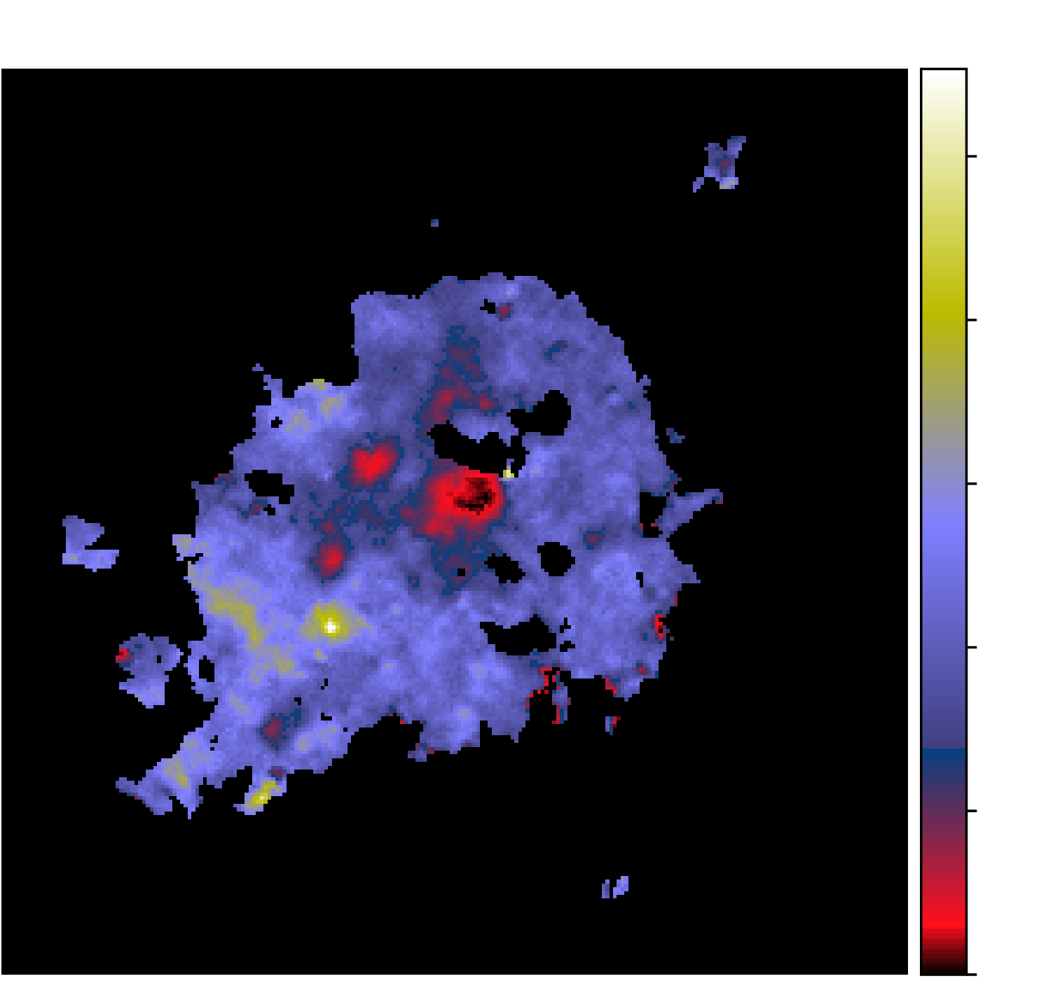
Evidence in resolved regions. This last point is observationally verified in countless regions. It can be conveniently witnessed, as the smallest grains are the carriers of the MIR continuum, which is well separated from the rest of the emission (cf. Fig. 2.27.b). In addition, small carbon grains carry the series of aromatic features (cf. Sect. 3.2.1.1). The disappearance of these features in regions of enhanced ISRF is very likely the sign of the destruction of these grains by hard UV photons. This is, for instance, evident in one of our studies of the massive star-forming region, N11, in the LMC (Galametz et al., 2016). This region contains several blobs, with embedded star clusters. The maps of the PAH mass fraction, (cf. Sect. 3.1.2.2), is shown in Fig. 4.12.a. It has been derived by modeling the spatially-resolved SED of Spitzer and Herschel images. Comparing this image to the mean starlight intensity in Fig. 4.12.b, we see that PAHs are strongly depleted in the blobs where is enhanced. The photodestruction is evident. In the case of this massive region, a bright star cluster such as N11B can clear PAHs out over a region of typically pc.
Aromatic features are severely depleted around star-forming regions.
 |  |
Another destruction mechanism is grain erosion and vaporization by collisions with energetic ions, either in coronal plasmas (thermal sputtering; K), or in shock waves (kinetic sputtering; km/s). There is an abundant literature on the subject (e.g. Draine & Salpeter, 1979; Dwek & Scalo, 1980; Tielens et al., 1994; Jones et al., 1996; Jones, 2004; Nozawa et al., 2006; Micelotta et al., 2010; Bocchio et al., 2012, 2014; Hu et al., 2019, see also the review by Dwek & Arendt, 1992). We start by discussing thermal sputtering in this section, and will review kinetic sputtering in Sect. 4.2.2.3.
Sputtering times. The evolution of a grain of radius, , and mass, , subjected to sputtering in a gas of density , can be expressed (e.g. Hu et al., 2019):
| (4.29) |
where we have hidden all the microphysics into the sputtering yield, . This quantity depends on: (i) the gas temperature, , in case of thermal sputtering; or (ii) the shock velocity, , in case of kinetic sputtering. A detailed derivation of can be found in Nozawa et al. (2006, Sect. 5). For our simple discussion, we will adopt their yields, for silicate and carbon grains, fitted by Hu et al. (2019). In the thermal case, the sputtering rate can be expressed as:
| (4.30) |
Fig. 4.13.a shows the lifetimes of grains in a coronal plasma. With Eq. (), in the HIM (cf. Table 3.6), typical grains (Eq. ) have lifetimes of: (i) Myr, for silicates; and (ii) Myr, for carbon grains. In the case of SN II blastwaves, grains stay in post-shock conditions for only yr. Dust destruction by thermal sputtering is thus not the dominant process in the shocked ISM.
Grains have short lifetimes in coronal plasmas.

Early-type galaxies. We have seen in Sect. 3.1.3.1 that ETGs tend to be characterized by a diffuse X-ray emission, originating in a permeating coronal gas. This HIM is likely filling most of their ISM. This has consequences on the dust properties. This can be seen in Fig. 4.14.a, looking at a classic scaling relation between the dustiness and the specific gas mass 6, . Most ETGs appear to be distributed on a vertical branch, below the main trend. They appear to be depleted in dust, at a given specific gas mass. Investigating the contribution of the X-ray emitting coronal gas, we have displayed the specific dust mass, as a function of the X-ray-luminosity-to-dust-mass ratio, , in Fig. 4.14.b (G21). The ratio quantifies the X-ray photon rate per dust grain. We see that ellipticals occupy the lower right corner of this relation: they have a high photon rate per dust grain and a low specific dust mass. We have just shown that grains in a hot gas have a short lifetime (Eq. ). The correlation of Fig. 4.14.b is thus likely the result of enhanced thermal sputtering in ETGs.
 |  |
We now focus on the effect of kinetic sputtering. This process leads to erosion and vaporization of grains in SN II blast waves. As we will see, this happens to be the major dust grain destruction mechanism. The kinetic sputtering rate is similar to the thermal case (Eq. ), except that the sputtering yield now depends on the shock velocity, (cf. Fig. 4.13.b):
| (4.31) |
In addition, grain shattering in grain-grain collisions is an important dust destruction mechanism in SN II blast waves (e.g. Kirchschlager et al., 2021).
Evidence in resolved regions. Although the efficiency of the process is debated, the reality of dust destruction by SN II shock waves is rather consensual. This process can even be observed in spatially-resolved SNRs. In particular, ISO and Spitzer MIR spectra of pre-shock and post-shock matter show systematic differences in, for instance: (i) 3C391 (Reach et al., 2002); (ii) SN1987A (Dwek et al., 2008; Arendt et al., 2016); and (iii) PuppisA (Arendt et al., 2010). The post-shock ISM exhibits:
Global model prescription. Similarly to what we did for grain growth (Eq. ), it is convenient to express the dust destruction rate as a function of global galactic quantities. Such a formula was proposed by Dwek & Scalo (1980):
| (4.32) |
where is the SN II rate (Eq. ), and is an empirical parameter quantifying the destruction efficiency. The latter represents the gas mass swept by a single SN II blast wave, within which all grains are destroyed. Eq. () can be understood the following way.
| (4.33) |
The destruction efficiency. The dust destruction efficiency, quantified by the parameter in Eq. (), ranges in the literature between and . It can be roughly estimated with the following arguments (Draine, 2009, slightly adapting his numbers):
This estimate corresponds to a dust lifetime of Myr, in the MW. This is a value close to what is found by more detailed, theoretical studies (e.g. Jones et al., 1996). Note however that a recent re-estimate, using hydrodynamical simulations, and accounting for the role of dust mantles found: (i) a shorter lifetime for carbon grains; but (ii) a significantly longer lifetime ( Gyr) for silicates (Slavin et al., 2015). We will give our own take on this timescale in Sect. 4.3.1.2.
A single SN II blast wave can destroy up to of dust, at Solar metallicity, resulting in a dust lifetime of Myr.
Cosmic dust evolution is the modeling of dust evolution from a global point of view, at the scale of a galaxy, over cosmic times 7. At galaxy-wide scales, most dust evolution processes can be linked to star formation: (i) formation of molecular clouds and their subsequent evaporation; (ii) stellar ejecta; (iii) SN shock waves; (iv) UV and high-energy radiation. The characteristic timescale of these processes is relatively short (of the order of the lifetime of massive stars; Myr) and their effect is usually localized around star-forming regions. For these reasons, the sSFR is an indicator of sustained dust processing. However, the dust lifecycle is a hysteresis. There is a longer term evolution, resulting from the progressive elemental enrichment of the ISM, which becomes evident on timescales of Gyr. This evolutionary process can be traced by the metallicity. Fig. 4.15 illustrates these two timescales by comparing the SEDs of a few galaxies.

We start by focussing on the build-up of the total dust mass. We will discuss the evolution of small carbon grains in Sect. 4.3.2. For terminological consistency of the rest of the discussion, let’s define the following metallicity regimes:
We will see in Sect. 4.3.1.2 that these ranges correspond to dust evolution regimes of nearby galaxies.
The first model accounting for the evolution of the gas content of galaxies and its cycle with star formation was presented by Schmidt (1959). The Eqs. 7-9 of Schmidt (1959) are the basic equations for the evolution of the gas mass as a result of the successive waves of star formation. Subsequent studies included the heavy element enrichment of the gas, therefore accounting for the chemical evolution of galaxies (e.g. Audouze & Tinsley, 1976, for an early review). Dwek & Scalo (1980) then initiated the first cosmic dust evolution model, by including grain processing in the gas enrichment modeling. Dwek (1998) modeled the radial trends in the MW, accounting for the individual elemental yields by stars of different initial masses. Such models have since then been refined (e.g. Morgan & Edmunds, 2003; Dwek et al., 2007; Zhukovska et al., 2008; Galliano et al., 2008a; Hirashita & Kuo, 2011; Asano et al., 2013; Rowlands et al., 2014; Zhukovska, 2014; Feldmann, 2015; De Looze et al., 2020; Galliano et al., 2021). These models are nowadays used to account for subgrid physics in numerical simulations of galaxy evolution (e.g. Hou et al., 2017; Aoyama et al., 2020).
Physical ingredients and assumptions. The different cosmic dust evolution models we have just cited above all have differences. They however have a common set of physical ingredients and assumptions. In what follows, we describe the model of G21, which is well representative of the diversity found in the literature.
| (4.34) |
The ejected masses. The dust evolution differential equations we will discuss below depend on the gas, heavy element and dust masses ejected by stars, at time :
| (4.35) |
These three equations are essentially the integral of the products of three terms: .
The equations of evolution. The physical ingredients and assumptions we have discussed earlier in this section translate into four coupled differential equations describing the temporal evolution of the stellar, gas, heavy element and dust masses, , , and :
Eqs. (-) simply express the time derivative of the mass, on the left-hand side, and the sum of the different individual rates on the right-hand side, some positive, some negative. We can note a few points.
Dust evolution tracks. We now present a set of solutions to Eqs. (-). For simplicity, we adopt the Chabrier IMF (Eq. ) and the delayed SFH (Eq. ). The total baryonic, initial mass of the galaxy is assumed to be . Fig. 4.16 shows the time evolution of the main quantities, for a MW-like galaxy. We have adopted the following parameters:
| (4.40) |
Fig. 4.16.a shows the SFH we have adopted. The time evolution of the individual quantities are represented in Fig. 4.16.b. We can note the following points.

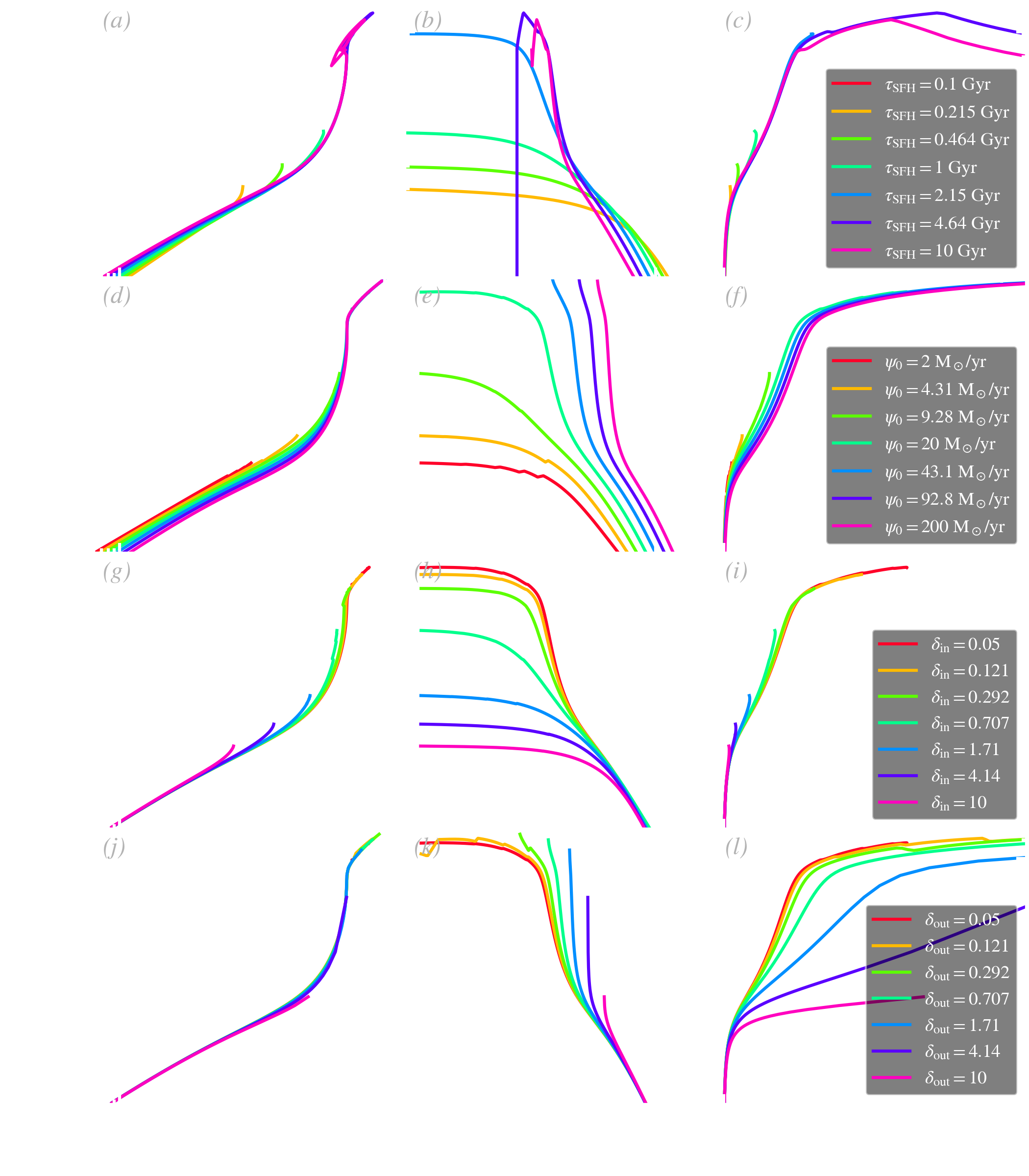
Effects of the individual parameters. We end this section by demonstrating the effects of the seven parameters of Eq. () on dust evolution. We vary each parameter, one by one, keeping the other ones to their values in Eq. (). We represent the dustiness, as a function of: (i) metallicity; (ii) sSFR; and (iii) gas fraction, . For completeness, we have represented the four SFH-related parameters in Fig. 4.17. Our center of interest is however the three dust evolution tuning parameters, represented in Fig. 4.18.
| (4.41) |
Since we usually have , we can write the rough proportionality: , with being a steep function of . This is the reason why the relative efficiency of the two processes is so strongly metallicity dependent.

We now discuss some empirical estimates of the three main grain evolution parameters (, and ), derived from fitting dust scaling relations. This is not a new topic. Several studies have attempted to tackle this issue (e.g. Lisenfeld & Ferrara, 1998; Morgan & Edmunds, 2003; Galliano et al., 2008a; Mattsson & Andersen, 2012; Rémy-Ruyer et al., 2014; De Vis et al., 2017; Nanni et al., 2020; De Looze et al., 2020). We have recently published such a study (G21). We will try to demonstrate the progress it has brought to the field.
Fitting dust scaling relations. We have used the SED modeling results of the DustPedia/DGS sample we have already discussed in Fig. 3.17 and Sect. 4.2.2.2 (G21). These results were obtained using the composite approach (Sect. 3.1.2.2), with the THEMIS grain properties, and a hierarchical Bayesian model (Sect. 5.3.3). These results are an estimate of: (i) the dust mass, , for all galaxies (G21); (ii) the stellar mass, and SFR for most of them (Rémy-Ruyer et al., 2015; Nersesian et al., 2019); (iii) the metallicity, , for about half the sample (Madden et al., 2013; De Vis et al., 2019). The dust evolution model of Sect. 4.3.1.1 has then been fitted to our estimates of , , , and SFR. We have adopted a hierarchical Bayesian approach (cf. Sect. 5.3.3), varying the following set of parameters.
Fig. 4.19 shows the fitted dustiness-metallicity relation, from our study (G21). We have represented the estimated observed quantities (SUEs) on top of the posterior PDF of our dust evolution model. This figure clearly shows the physical origin of the three regimes we had arbitrarily defined at the beginning of Sect. 4.3.1.
| (4.42) |
| (4.43) |

Evolutionary timescales as a function of metallicity. The dust evolution fitting of Fig. 4.19 allowed us to infer the values of the three tuning parameters. Accounting for possible systematic biases, we concluded the following (G21):
| (4.44) |
These efficiencies can be translated into timescales of the three dust evolution processes, in each galaxy. We have represented these timescales as a function of metallicity, in Fig. 4.20. The derived timescales for the MW are represented as a yellow star, although they were not used in the fit. We note the following points
| (4.45) |
| (4.46) |
The two processes thus balance each other around . This is where our value of the critical metallicity comes from. We note that, for the MW, we find Myr and Myr, close to the values we had expected in Sect. 4.2.1.3 and Sect. 4.2.2.3. Yet, we did not put any prior on the Galactic values. This is a indication in favor of the consistency of our analysis.
| (4.47) |
SN II are net dust destroyers, except at very low metallicity.

Methodological remarks. The study this section relies on (G21) was the first rigorous empirical determination of the dust evolution tuning parameters in Eq. (), using a wide enough metallicity range to unambiguously constrain these quantities. We emphasize two important points.
The controversy about stardust. We have opened this chapter with a citation of D09, about the belief that ISD could be mainly stardust. It is unfortunate that this discussion can sometimes turn into an ideological debate, in the literature.
To try to rise above a mere ideological debate, we should not lose sight of the big picture, as the truth is the whole. Table 4.2 summarizes the observational evidence in favor of one scenario and the other.
|
| Stardust | ISM |
|
| origin | origin |
| Elemental depletions (cf. Sect. 2.2.3 & Sect. 4.2.1.1) | ||
| Nearby galaxy dustiness-metallicity trend (cf. Sect. 4.3.1.2) | ||
| Individual SNRs (before the reverse shock; cf. Sect. 4.1.2.2) | ||
| Individual SNRs (accounting for the reverse shock; cf. Sect. 4.1.2.2) | ||
| Isotopic ratios of IDPs in meteorites (cf. Sect. 4.1.2.2) | ||
| Distant dusty galaxies (cf. Sect. 4.3.1.2) | ||
| DLA dustiness-metallicity trend (cf. Sect. 4.3.1.2) | ||
| ISD is mainly amorphous, while CSD is crystalline (cf. Sect. 4.1.2.2) | ||
| Emissivity variation as a function of ISM density (cf. Sect. 4.2.1.1) | ||
|
|
Limitations of our approach. Although our approach was successful in providing a unique, rigorous estimate of the dust evolution tuning parameters, and in deriving timescales as a function metallicity, it has several limitations.
We close this chapter with a discussion about the trend followed by the grains carrying the aromatic feature emission. We have already discussed this point in Sect. 3.2.1.4, from a spectroscopic point of view. We now give a more general point of view, based on SED modeling, and discuss the different scenarios. We remind the reader that aromatic features can be emitted by PAHs 9 or small a-C(:H)s. This is a debated modeling choice (cf. Sect. 2.3). In the present section, we will assume that small a-C(:H)s are the carriers. Their mass fraction is (cf. Sect. 2.3.3.1). Small a-C(:H) and PAHs emit similar aromatic feature strengths if (G21).
Aromatic features are significantly weaker in low-metallicity systems, compared to normal galaxies (cf. Sect. 3.2.1.4). This fact could indicate an increasing formation efficiency as a function of . However, low-metallicity environments have also their ISM bathed with a hard, permeating ISRF (cf. Sect. 3.3.2.3). Knowing that small a-C(:H)s are massively destroyed by such an ISRF (cf. Sect. 4.2.2.1), this trend could result from the increased suppression of aromatic features at low metallicity. Several scenarios have been proposed to explain these trends.
Enhanced destruction at low metallicity. Madden et al. (2006) proposed that small a-C(:H)s are more efficiently destroyed at low metallicity. This was supported by the relation in Fig. 3.41, between the strength of the aromatic features and the [Ne III]/[Ne II] tracing the hardness of the ISRF. The fact that dwarf galaxies have in general harder, more intense ISRF is linked to the following facts.
Another mechanism, proposed by O’Halloran et al. (2006), is the destruction of aromatic feature carriers by SN II blast waves. However, this scenario is less satisfactory, as blast waves tend to destroy all dust species (e.g. Reach et al., 2002). They therefore do not constitute a consistent explanation for the selective destruction of small a-C(:H)s.
Inhibited formation efficiency at low metallicity. Several scenarios based on metallicity-dependent production mechanisms, in stellar ejecta or in the ISM, have been proposed.
G21 have derived in each galaxy of the DustPedia/DGS sample, that we have already amply discussed earlier in this chapter. Fig. 4.21 shows the evolution of this quantity with: (a) the metallicity, ; and (b) the mean starlight intensity, (Eq. ).

A better correlation with metallicity. Fig. 4.21.a shows a clear linear rising trend of with metallicity (Eq. 9 of Galliano et al., 2021), and a decreasing trend of , with quantifying the intensity of the ISRF. Both correlations could be explained by any of the scenarios discussed in Sect. 4.3.2.1. We have however found that the correlation with metallicity is significantly better (cf. detailed discussion in Sect. 4.2.2 of Galliano et al., 2021). This result is worth noting, especially since several studies focussing on a narrower metallicity range concluded the opposite (e.g. Gordon et al., 2008; Wu et al., 2011). It probably relies on the fact the metallicities we have adopted in this study (De Vis et al., 2019) correspond to well-sampled galaxy averages, while in the past a single metallicity, often central, was available and may have not been representative of the entire galaxy. This result suggests that photodestruction, although real at the scale of star-forming regions, might not be the dominant mechanism at galaxy-wide scales and that one needs to invoke one of the inhibited formation processes discussed in Sect. 4.3.2.1.
At global scales, the mass fraction of small a-C(:H) seems to correlate better with metallicity than with the ISRF.
The global point of view. Overall, the trend might have several origins. We think we can be confident about the following facts.
What makes this question difficult to tackle is the diversity of spatial scales needed to properly balance the different processes. Ideally, we would indeed need to account for the following.
To know the origin of the trend, we would need to reliably estimate the contribution to the integrated emission of both of these components, resolving sub-pc scales, in order to account for the enhanced emissivity in PDRs. This is out of reach of current facilities.

The potential of quiescent very-low-metallicity galaxies. An alternative would be to observe quiescent very-low-metallicity systems. We know such a population of galaxies exist (e.g. Lara-López et al., 2013). Let’s assume that we can estimate for a galaxy with and . We have represented the two possible solutions on Fig. 4.22. We see that:
Such observations would require a sensitive MIR-to-FIR observatory, such as what SPICA (van der Tak et al., 2018) could have been.
1.In thermonuclear reactions, the high temperature gives nuclei enough kinetic energy to overcome their Coulomb barrier, and allows them to fuse with each other.
2.The Sun’s core is at K.
3.The degeneracy pressure is due to the fact that fermions can not occupy the same state. In very dense environments, this leads to a pressure: electron degeneracy pressure in white dwarfs; neutron degeneracy pressure in neutron stars.
4.Careful though, some authors quote IMFs, normalized as .
5.As a reminder, the metallicities of the Magellanic clouds are: and (Pagel, 2003).
6.Given an extensive quantity, , it is common, in extragalactic astronomy, to define the corresponding intensive specific quantity, , by dividing by the stellar mass.
7.We assume that the age of the Universe is Gyr (e.g. Hogg, 1999).
8.The sawtooth features in Fig. 4.18.d-f, for the two lowest values of (red and orange), are numerical artefacts due to the fact that grain growth is so low, that SN II can clear dust faster than our time resolution.
9.Alternative acronym: Poor-people’s Amorphous Hydrocarbon...