1 Propaedeutics in Dust Physics

Chapter 1
Propaedeutics in Dust Physics

1.1 The Make-Up of Solids
  1.1.1 Atomic Structure
   1.1.1.1 The Hydrogen Atom
   1.1.1.2 Polyelectronic Atoms
   1.1.1.3 The Valence Shell
   1.1.1.4 Orbital Hybridisation
  1.1.2 Molecular Bonding
   1.1.2.1 Covalent Bonds
   1.1.2.2 Ionic Bonds
   1.1.2.3 Metallic Bonds
   1.1.2.4 Intermolecular Attraction
  1.1.3 The Solid State
   1.1.3.1 The Different Types of Solids
   1.1.3.2 The Band Structure of Solids
   1.1.3.3 The Fermi Level
  1.1.4 Interstellar Dust Candidates
   1.1.4.1 Silicates
   1.1.4.2 Hydrogenated Amorphous Carbon
   1.1.4.3 Graphite
   1.1.4.4 Polycyclic Aromatic Hydrocarbons (PAH)
1.2 The Interaction of Light with Solids
  1.2.1 Bonds as Harmonic Oscillators
   1.2.1.1 The Harmonic Oscillator Amplitude
   1.2.1.2 The Plasma Frequency
   1.2.1.3 The Dielectric Function
   1.2.1.4 Harmonic Oscillator Cross-Section
   1.2.1.5 Optical Constants of Conductors
   1.2.1.6 The Kramers-Kronig Relations
  1.2.2 Grain Optical Properties
   1.2.2.1 Why Are Most Dust Features in the MIR?
   1.2.2.2 Dielectric Functions of Realistic Materials
   1.2.2.3 Computing Grain Cross-Sections
   1.2.2.4 Beyond Homogeneous Spheres
   1.2.2.5 Polarization
  1.2.3 Heat Capacities
   1.2.3.1 Distribution of Harmonic Oscillators
   1.2.3.2 Debye’s Model
   1.2.3.3 Heat Capacities of Realistic Materials
  1.2.4 Heating and Cooling
   1.2.4.1 Kirchhoff’s Law
   1.2.4.2 Equilibrium Heating
   1.2.4.3 Stochastic Heating
   1.2.4.4 Collisionnal Heating

As soon as we thought something, look in what sense the opposite is true.

(Simone WEIL; Weil, 1947)

Most reviews about ISD (e.g. Draine, 2003a; Whittet, 2003; Tielens, 2005; Draine, 2011; Jones, 2016a,b,c; Galliano et al., 2018) assume that the reader has a good knowledge of solid-state physics ¹. It is however not always the case, especially among students. The present chapter is intended to synthesize the basic knowledge necessary to understand contemporary publications in the field. We have opted for a simple presentation of the most important concepts, accompanied with a few original figures. We present the most important formulae and refer the reader to reliable textbooks for their proofs. We have tried to answer everything students always wanted to know about dust, but were afraid to ask.

1.1 The Make-Up of Solids

Atoms can be combined to form molecules or solids. The properties of these compounds depend greatly on the way their constitutive atoms are bonded together, by their electrons. Electrons being fermions (their spin is 1/2), the Pauli exclusion principle implies that each of them must occupy a different state in a system, characterized by its wave function (e.g. Tome II, Chapter XIV of Cohen-Tannoudji et al., 1996). The electronic shells of atoms, the bonds of molecules and the band structure of solids all follow from this principle.

1.1.1 Atomic Structure

1.1.1.1 The Hydrogen Atom

The electrons of an atom each have a distinct wave function, $Ψ$ , called orbital. The probability density function of presence of the electron is proportional to $| Ψ |^{2}$ . These orbitals are solutions to the Schrödinger equation, in the electrostatic well created by the nucleus, assumed to be infinitely heavy ². These solutions are relatively simple in the case of the hydrogen atom (cf. e.g. Chap. 3 of Bransden & Joachain, 1983). Its single electron can occupy different shells, characterized by their principal quantum number, $n$ . This quantum number determines the energy level of the orbitals ( $E \propto 1 ∕ n^{2}$ ) as well as their size (cf. Table 1.1). Each individual shell is divided into subshells, characterized by the azimuthal number, $l$ , quantifying the angular momentum of the electron ( $L \propto \sqrt{l (l + 1)}$ ), which can be 0, for s subshells (cf. Table 1.2). The orbitals in each subshell are combinations of spherical harmonic functions. These functions are anisotropic. The magnetic quantum number, $m_{l}$ , quantifies their orientation in space, as displayed in Fig. 1.1. Finally, the spin quantum number, $m_{s}$ , quantifies the direction of the electronic spin (up or down).


Name	Symbol	Values	Signification

Principal	$n$	$1, 2, \dots, \infty$	Energy ( $E \propto 1 ∕ n^{2}$ for H) or size of the shell

Azimuthal	$l$	$0, 1, \dots, n - 1$	Angular momentum ( $L \propto \sqrt{l (l + 1)}$ )

Magnetic	$m_{l}$	$l, l - 1, \dots, - l$	Orientation (spherical harmonic combination)

Spin	$m_{s}$	$+ 1 ∕ 2, - 1 ∕ 2$	Magnetic moment (spin direction)

Table 1.1: Atomic quantum numbers. Adapted from Table 7.2 of Atkins (1992).


Principal	Bohr	Azimuthal quantum number
quantum	shells	s	p	d	f	Subshell letter
number		2	6	10	14	Number of electrons per subshell

$n = 1$	K	$l = 0$

$n = 2$	L	$l = 0$	$l = 1$

$n = 3$	M	$l = 0$	$l = 1$	$l = 2$

$n = 4$	N	$l = 0$	$l = 1$	$l = 2$	$l = 3$

Table 1.2: Atomic shell structure. We have highlighted the correspondence with the shells of Bohr’s pre-quantum atomic model. The letters s, p, d, f are used to label orbitals with different values of

l

Figure 1.1: Shape of s, p, d, f electron orbitals. These shapes represent the surfaces encompassing the region where the electron has a $90 %$ probability of presence. The orbitals are identified by the letter corresponding to the value of $l$ (cf. Table 1.2), with the value of $m_{l}$ as an index. Credit: UCDavis Chemwiki, licensed under CC BY-NC-SA 3.0 US.

1.1.1.2 Polyelectronic Atoms

The different energy levels of an atom can be populated by excitation (collision or photon absorption). In the fundamental state of the H atom, the electron occupies the $n = 1$ level. The electrons of a polyelectronic atom in its fundamental state occupy the lowest energy orbitals available. Each electron must have a unique set of the four quantum numbers (Table 1.1). The nucleus charge, $Z$ , is higher, which causes the inner shells to be closer to the nucleus. The electric field seen by the outer shells is thus partially screened by the inner shells. A fundamental difference between polyelectronic atoms and hydrogen is however the mutual repulsion of the electrons (cf. e.g. Chap. 7 of Bransden & Joachain, 1983). The different subshells (s, p, d, f) of a given shell having different geometries, the mutual repulsion depends on $l$ . The subshells of a given $n$ thus have different energies. The electronic configuration of atoms in their fundamental state results from the ranking in energy of these levels. The possible number of electrons per subshell is given in Table 1.2. We have represented the electronic configuration of atoms in the periodic table (Fig. 1.2).

Figure 1.2: Periodic table of elements. We show only the first four rows, as they contain all the elements relevant to ISM physics. Z is the charge and A, the atomic weight. In each cell, we show the electronic configuration in the fundamental state. We do not repeat the part of the configuration corresponding to the noble gas of the previous row ([He], [Ne], [Ar]). We have annotated the table with the four quantum numbers of the last electron. Licensed under CC BY-SA 4.0.

1.1.1.3 The Valence Shell

The outer shell is called the valence shell. It contains the electrons responsible for molecular bonds (cf. Sect. 1.1.2) and shaping the optical properties of solids (cf. Sect. 1.2). We will see that the nature of the chemical bond depends on the tendency of its atoms: (i) to share electrons; (ii) to form cations, by losing one or several electrons; or (iii) to form anions, by gaining one or several electrons.

Ionization potential. Panel (a) of Fig. 1.3 shows the first ionization potential, $I_{1}$ , of the elements in Fig. 1.2. Atoms with a low $I_{1}$ tend to form stable cations. Noble gases have the largest $I_{1}$ of their row, because their last shell is full. More generally, Fig. 1.3 shows that $I_{1}$ increases from the left to the right of the periodic table (Fig. 1.2), as the valence shell gets fuller. This is because, at a given $n$ , moving to the right of the table increases the effective nucleus charge $Z - Z_{s u b s h e l l s}$ , making the valence shell more tightly bound. It also decreases from the top to the bottom, as the energy level of the outer shell decreases with $n$ as $1 ∕ n^{2}$ .

$\Rightarrow$ Metals tend to form stable cations.

Electron affinity. Panel (b) of Fig. 1.3 shows the first electron affinity, $A_{1}$ , of the elements in Fig. 1.2. Atoms with a high electron affinity tend to form stable anions. $A_{1}$ follows roughly the same trend as $I_{1}$ , with some exceptions. Noble gases have their last shell full, they therefore tend to remain neutral and have a negative $A_{1}$ . Alkaline earth metals also have negative $A_{1}$ , because of the energy difference between their full $n$ s and empty $n$ p shells.

$\Rightarrow$ Non metals tend to form stable anions.

Electronegativity. The balance between $I_{1}$ and $A_{1}$ gives an idea of the tendency of an atom to attract electrons in a bond. Mulliken’s electronegativity, $χ$ , is defined as (e.g. Huheey et al., 1993):

χ = 0.187 \times (\frac{I_{1}}{1 eV} + \frac{A_{1}}{1 eV}) + 0.17 .

(1.1)

If we except noble gases, we see that $χ$ will be higher to the right of the periodic table, and will decrease from the top to the bottom.

Figure 1.3: First ionization potentials and electron affinities. In panel (a), we display the first ionization potential. It is the minimum energy required to expel the most loosely bound electron, in the fundamental state. It is the energy lost during the gas phase reaction: $X \to X^{+} + e^{-}$ . In panel (b), we display the first electron affinity, which is the energy gained by adding an electron to the atom. It is the energy released during the gas phase reaction: $X + e^{-} \to X^{-}$ . Elements with a negative electron affinity (yellow hatched area) do not form stable anions. We display the different groups with the same color code as in Fig. 1.2. Licensed under CC BY-SA 4.0.

1.1.1.4 Orbital Hybridisation

To explain the shape of molecules, the concept of hybrid orbitals was introduced in the 1930’s by Linus PAULING. The principle is that orbitals with similar energies can be linearly combined together to form new orbitals with different shapes ³. The most relevant example to ISD is the hybridisation of carbon. A 2s electron can be promoted to 2p, resulting in the following configuration.

The carbon is now in an excited state, noted C $^{*}$ . The promotion requires 4.2 eV. From this new state, the following combinations of orbitals are possible.

sp $^{3}$ hybrids: are 1/4 s and 3/4 p. This hybridisation results in four sp $^{3}$ orbitals arranged in a tetrahedron, shown in Fig. 1.4.a. For instance, C in methane (CH $_{4}$ ) is sp $^{3}$ hybridized. The electronic configuration of the $n = 2$ shell becomes the following.
sp $^{2}$ hybrids: are 1/3 s and 2/3 p. This hybridisation results in one standard p orbital and three sp $^{2}$ orbitals trigonally-arranged, shown in Fig. 1.4.b. For instance, C in benzene (C $_{6}$ H $_{6}$ ) is sp $^{2}$ hybridized. The electronic configuration of the $n = 2$ shell becomes the following.
sp hybrid: is 1/2 s and 1/2 p. This hybridisation results in two standard p orbitals and two sp orbitals linearly-arranged, shown in Fig. 1.4.c. For instance, C in acetylene (C $_{2}$ H $_{2}$ ) is sp hybridized. The electronic configuration of the $n = 2$ shell becomes the following.

Figure 1.4: Hybrid orbitals of carbon. The left image shows the shape of the four sp $^{3}$ orbitals of a C atom. They are arranged in a tetrahedral geometry. The center image shows the shape of the three sp $^{2}$ orbitals of a C atom. They are arranged in a trigonal geometry. We have not displayed the remaining p orbital of this C atom. The right image shows the shape of the two sp orbitals of a C atom. They are arranged along a line. We have not displayed the remaining two p orbitals of this C atom. Each bond is represented with a black line indicating its direction: (i) thin solid lines show bonds within the plane of the image; (ii) the thick solid line shows a bond pointing toward the reader; (iii) the dashed line shows a bond pointing in the opposite direction. Credit: adapted from Wikipedia’s Orbital hybridisation article (changed the central letter), licensed under CC BY-SA 3.0.

1.1.2 Molecular Bonding

Chemical bonds are the result of the overlap between the outer orbitals of two atoms whose valence shell is not full (cf. e.g. Chap. 8 of Atkins, 1992). Despite their mutual repulsion, sharing electrons leads to a lower energy state, in which a stable bonded molecule is formed. Covalent, ionic and metallic bonds, that we will define below, typically have dissociation energies of a few eV. The atomic spacing in a molecule or a solid is of the order of a few Å.

Figure 1.5: Different types of molecular bonds. We have noted $\vec{p}$ , the dipole moment created by the bond. In general, $\vec{p} = ∭_{V} \vec{r} . ρ (\vec{r}) d V$ , where $ρ (\vec{r})$ is the charge number density. In the case of MgO, it reduces to $e . \vec{O.Mg}$ , where $\vec{O.Mg}$ is the distance vector between the two ions. The electrons are noted $e^{-}$ , and $δ^{+}$ and $δ^{-}$ are the excess dipolar charges of both signs. Licensed under CC BY-SA 4.0.

1.1.2.1 Covalent Bonds

A covalent bond is formed when a pair of electrons with anti-parallel spin is shared between two atoms of similar electronegativity. The more the orbitals overlap, the stronger the bond is. The electron density is the highest between the two atoms, resulting in a directional bond. For instance, the H₂ (Fig. 1.5.a) and CO molecule bonds, as well as the C-C and C-H bonds in hydrocarbons, are all covalent. Covalent bonds are weakly polar. Symmetric molecules such as H₂ are non-polar, whereas asymmetric molecules, such as CO are polar, because of the difference in electronegativity of C and O.

$\Rightarrow$ Covalent bonds are preferentially formed between non metals.

Covalent bonds are of one of the two following types.

$σ$ bonds: result from the frontal overlap of two s, p or sp $^{n}$ ( $n = 1, 2, 3$ ) orbitals. These bonds have a rotational symmetry around their axis (Fig. 1.6.a). The electron density is maximum between the two atoms. It is the strongest covalent bond. The C–C bond of ethane (C $_{2}$ H $_{6}$ ) is a $σ$ bond.
$π$ bonds: result from the side-by-side overlap of the two lobes of two p orbitals (Fig. 1.6.b). The electron density is maximum above and below the plane of the molecule and zero between them. These bonds are weaker than $σ$ bonds. In the double C $=$ C bond of ethylene (C $_{2}$ H $_{4}$ ), there are one $σ$ and one $π$ bonds (Fig. 1.6). In the triple C $\equiv$ C bond of acetylene (C $_{2}$ H $_{2}$ ), there are one $σ$ bond and two $π$ bonds.

Finally, some transitions in interstellar solids involve antibonding orbitals. When a bond forms, both a bonding and an antibonding molecular orbitals with different energy levels become available. This is demonstrated for the H $_{2}^{+}$ molecule, with the Schödinger equation, in Chap. 9 of Bransden & Joachain (1983). Bonding orbitals have a lower energy level than the dissociated atoms, thus favoring a stable molecule. On the contrary, the population of an antibonding orbital makes the molecule unstable. For instance, the splitting of molecular orbitals for both $σ$ and $π$ bonds of ethylene (Fig. 1.6) are the following.

We emphasize those are electronic levels of molecules. Molecules also have rotational and vibrational modes that will be discussed in Sect. 1.2.2.1.

Figure 1.6: An example of $σ$ and $π$ bonds. We demonstrate the two types of bonds on ethylene (C $_{2}$ H $_{4}$ ). On the left image: the s orbital of each H atom is shown in red; the p orbital of each C atom is shown in green; and the three sp $^{2}$ hybridized orbitals of each C atom are in orange. The frontal overlap of the sp $^{2}$ hybridized orbitals of two C atoms, as well as the overlap of one sp $^{2}$ hybridized C orbital with the s orbital of an H atom, both form a $σ$ bond. On the middle image, we show the plane of the molecule with the p orbital of each C atom in green. The right image shows the overlap of these two p orbitals to form one single $π$ bond, in blue, on both sides of the plane. Credit: adapted from the Chemistry Library, licensed under CC BY-NC 4.0.

1.1.2.2 Ionic Bonds

An ionic bond is formed between two atoms of significantly different electronegativities. The electron is transferred from the cation to the anion, resulting in a polar bond. The adhesion is due to long-range Coulomb forces ( $\propto 1 ∕ r^{2}$ ) between the two ions. Ionic bonding is non-directional as the electron cloud stays centered around the atoms. The most relevant example to ISD is the O $^{2 -}$ –Mg $^{2 +}$ bond in silicates (Fig. 1.5.b).

$\Rightarrow$ Ionic bonds are preferentially formed between a metal and a non metal.

Covalent and ionic bonds are two extreme cases. Most bonds involving at least one non metal are intermediate between both.

1.1.2.3 Metallic Bonds

Metals can easily be ionized. Bonding several metal atoms therefore results in a lattice of cations bathed in a sea of free valence electrons. The electrons are not attached to a particular atom and can be found anywhere in the solid. This explains the electric and thermal conductivities of metals. Fig. 1.5.c represents solid iron.

$\Rightarrow$ Metallic bonds are formed between a large number of metal atoms.

1.1.2.4 Intermolecular Attraction

Weaker forms of attraction between molecules exist. Their dissociation energy is typically of the order of $≃ 0.1$ eV. They are relevant to ISD studies.

Van der Waals bonds: are due to the induced dipole attraction of neutral atoms and molecules. Their potential energy drops as $1 ∕ r^{6}$ . They are in particular responsible for binding graphene sheets together in graphite (Fig. 1.5.d).
Hydrogen bridges: are formed when the induced dipole of the H atom of a molecule is attracted by the induced dipole of a strongly electronegative atom in another molecule. For instance, hydrogen bridges tie the H $_{2}$ O molecules together in water ice (Fig. 1.5.e).

1.1.3 The Solid State

1.1.3.1 The Different Types of Solids

There are two main types of solids: insulators and conductors. Their properties are radically different. Their difference originates in the type of chemical bond making up their crystal lattice.

Insulators,: also called dielectrics, are solids, whose atoms are tied together with covalent or ionic bonds. The valence electrons are therefore located around their specific atoms and can not move freely through the lattice. Consequently, when an electric field is applied, it induces a polarization of the bonds, distorting them, but no current is flowing. For instance, silicates are dielectric materials.
Conductors: are solids, whose atoms are tied together with metallic bonds. Their valence electrons are therefore free to move through the solid. Consequently, when an electric field is applied, a current is flowing. For instance, iron is a metallic conductor. There are a few non-metal conductors, such as graphite, which is classified as a semimetal. This peculiar property is due to the delocalized electrons within the aromatic cycles constituting graphite (cf. Sect. 1.1.4).

There is a third, intermediate type of solids, called semiconductors. Semiconductors are insulators at $T = 0$ K and conductors at ambient temperatures. Several cosmic dust candidates belong to this category. We will define it more precisely in Sect. 1.1.3.3.

1.1.3.2 The Band Structure of Solids

A solid can be idealized as a periodic lattice of atoms bonded to each other. The permitted energy levels of a single valence electron, in the periodic electrostatic potential created by this lattice, are a series of continuous functions, also called bands (e.g. Chap. 8 of Ashcroft & Mermin, 1976, for a derivation from the Schrödinger equation). This can be viewed as a generalization of the molecular level splitting (Fig. 1.7). The spacing between a large number of levels is so small that it appears continuous. At $T = 0$ K, the lowest energy bands are filled in priority. Two of these bands are particularly important.

The valence band: is the highest energy band populated by valence electrons, at $T = 0$ K.
The conduction band: is the lowest energy band where electrons can move freely through the solid. It is the band immediately superior to the valence band.

The energy difference between the top of the valence band and the bottom of the conduction band is called the band gap, noted $E_{g}$ (Fig. 1.7).

Figure 1.7: Origin of the band structure of a solid. From the left to the right, we represent: (i) typical discrete atomic levels, (ii) the successive splitting of molecular orbitals, (iii) resulting in the quasi continuous distribution of levels in bands. Electrons are represented with a vertical blue arrow (up or down), corresponding to their spin. Licensed under CC BY-SA 4.0.

1.1.3.3 The Fermi Level

The probability distribution of identical fermions, such as electrons in a solid, over the energy states of a system at temperature $T$ , is given by the Fermi-Dirac distribution:

f (E) = \frac{1}{\exp (\frac{E - E_{F}}{k T}) + 1},

(1.2)

where $k$ is the Boltzmann constant (cf. Table B.2), $E$ denotes the different energy levels and $E_{F}$ is the Fermi level ⁴. This distribution is displayed in Fig. 1.8.a. The Fermi level is an intrinsic quantity characterizing a solid. It is the energy required to add an electron to the system. It also corresponds to the maximum energy an electron can have at $T = 0$ K. The latter interpretation of $E_{F}$ can be seen in Fig. 1.8.a. The blue curve shows Eq. ( $1.2$ ) at $T = 0$ K: (i) it gives equal probability to electrons to occupy energy levels $E \leq E_{F}$ ; (ii) it gives zero probability to energy levels $E > E_{F}$ . The actual number density of electrons, $n_{e}$ , is:

n_{e} = \int_{- \infty}^{\infty} g (E) f (E) d E,

(1.3)

where $g (E)$ is the density of states per infinitesimal energy bin. This density of states corresponds to the band structure. It is 0 between the bands. We emphasize that $E_{F}$ can fall between two bands. It does not necessarily correspond to an actual allowed level. This is demonstrated in Fig. 1.8.

Insulators: have their valence and conduction bands widely spread apart (Fig. 1.8.b). At ambient temperature, no electron will populate the conduction band. It is another way to see that their valence electrons are localized around their cations.
Semiconductors: have their valence and conduction bands close to each other (Fig. 1.8.c). They are insulators at $T = 0$ K, but their conduction band can be populated at ambient temperature ( $E_{g}$ gets closer to $k T$ ).
Conductors: are solids for which the valence and the conduction bands are the same (Fig. 1.8.d). The Fermi level is within the band. It is another way to see that the valence electrons are free to move through the lattice at any temperature.

Figure 1.8: The Fermi level and the different types of solid. The left plot shows the rotated Fermi-Dirac distribution (Eq. $1.2$ ), for two values of the temperature, $T = 0$ K and $T ≃ 300$ K. The three diagrams on the right show the valence and conduction bands relative to the Fermi level, $E_{F}$ , for insulators, semiconductors and conductors. For conductors, the valence band is also the conduction band. Licensed under CC BY-SA 4.0.

1.1.4 Interstellar Dust Candidates

We briefly review here the constitution of the most likely ISD grain candidates. Some general properties are given in Table 1.3. Their optical properties are extensively discussed in Sect. 1.2.2.

1.1.4.1 Silicates

The different types of silicates are built around silica tetrahedra (SiO $_{4}^{4 -}$ ), paired with various cations to produce a neutral compound (cf. e.g. Henning, 2010, for a review). The silica tetrahedra have a central Si $^{4 +}$ cation tied to four O $^{2 -}$ anions with covalent/ionic bonds. In the ISM, the most widely available divalent cations that can be paired with silica tetrahedra are Mg $^{2 +}$ and Fe $^{2 +}$ (cf. Sect. 2.2.3). Silicates have two strong features at 9.7 $μ m$ (Si–O stretching) and 18 $μ m$ (O–Si–O bending). They are ubiquitous: (i) they are the main constituent of Earth’s crust; (ii) they are also found in Solar system and CircumStellar Dust (CSD); (iii) they account for probably 2/3 of interstellar grain mass (e.g. Draine, 2003a); (iv) their features are observed in distant galaxies, in absorption (e.g. Marcillac et al., 2006) and in emission (e.g. Hony et al., 2011). Interstellar silicates are widely amorphous (e.g. Kemper et al., 2004). Crystalline silicates have additional distinctive narrow features, due to SiO $_{4}$ as well as (Fe,Mg)–O vibrations, in the 9.0–12.5 $μ m$ and 14-22 $μ m$ ranges, with a few bands above 33 $μ m$ . The following two types of silicates are the most relevant to ISD (cf. Table 1.3).

Olivine. Olivine have the general formula (Mg,Fe) $_{2}$ SiO $_{4}$ , with different proportions of Mg and Fe. Its crystalline structure is represented on Fig. 1.9.b. The two following compounds are the extreme cases of the Fe-to-Mg ratio.

Forsterite: is the Mg-end of the series, with formula Mg $_{2}$ SiO $_{4}$ .
Fayalite: is the Fe-end of the series, with formula Fe $_{2}$ SiO $_{4}$ .

Olivine have an olive green color (Fig. 1.10.a).

Pyroxene. Pyroxene have the general formula (Mg,Fe)SiO $_{3}$ , with different proportions of Mg and Fe. They are constituted of silica tetrahedron chains, sharing one O atom (Fig. 1.9.c), which explains their stoichiometry. The two following compounds are the extreme cases of the Fe-to-Mg ratio.

Enstatite: is the Mg-end of the series, with formula MgSiO $_{3}$ .
Ferrosilite: is the Fe-end of the series, with formula FeSiO $_{3}$ .

Pyroxene can be darker than olivine (Fig. 1.10.b).

$\Rightarrow$ In general, silicates are translucent minerals. They are gemstones, used in jewelry.

Figure 1.9: Structure of interstellar dust candidates. The (a) image shows the silica tetrahedron, which is the building block of silicates. The (b) image shows the structure of crystalline olivine. Some silica tetrahedra are pointing toward the reader above the yellow plane, and some are pointing backward. The latter appear dimmer and the Si atom are visible in red. The (c) image shows the structure of crystalline pyroxene. Its most important feature is the chain of alternate silica tetrahedra. They share one O atom, explaining why the stoichiometry of pyroxene is different from olivine. The (d) image shows the diversity of carbon pairing in an a-C(:H). Every C atom is sp $^{2}$ hybridized, except the aliphatic C, which is sp $^{3}$ hybridized. Every bond is a $σ$ bond except: (i) the 6 delocalized electrons within each aromatic cycles are $π$ bond pairing of p orbitals; (ii) one of the olefinic bonds is a $π$ bond. The example we have shown corresponds to a very small grain. In a larger a-C(:H), most of these bonds would be linked into the rest of a contiguous 3D network (e.g. Micelotta et al., 2012, for more realistic structures). The (e) image shows that graphite is the stack of graphene sheets. Each graphene sheet is made exclusively of aromatic cycles. The (f) image displays a few different PAHs. Licensed under CC BY-SA 4.0.

Figure 1.10: Appearance of various minerals. The (a) and (b) images show crystalline silicates. The soot powder (c) is an approximate analog of a-C(:H), on the a-C end, except that soot can contain radicals with O, N, etc. These images are useful to visualize the differences in optical properties of these compounds. They however show macroscopic samples. Even the powder in image (c) is made of particles much larger than 1 $μ m$ , which is the maximum size of interstellar grains. Credit: (a) forsterite from Rob LAVINSKY, licensed under CC BY-SA 3.0; (b) enstatite from Rob LAVINSKY, licensed under CC BY-SA 3.0; (c) soot from Wikipedia, not licensed; (d) graphite from Rob LAVINSKY, licensed under CC BY-SA 3.0; (e) PAHs from the Astrochemistry Lab, NASA Ames Research Center, with permission from Lou ALLAMANDOLA.

1.1.4.2 Hydrogenated Amorphous Carbon

This is a broad class of solids, noted a-C(:H) (a notation introduced by Jones, 2012b). Carbon atoms can be paired in the following ways (Fig. 1.9.d).

Aromatic cycles: are hexagonal rings made of six sp $^{2}$ hybridized C atoms. Two of the three available sp $^{2}$ orbitals of each C atom make $σ$ bonds, tying the cycle together. The last sp $^{2}$ orbital can be used to make a $σ$ bond with another C atom, extending the compound, or with an H atom, ending the solid in this direction. The six remaining p orbitals of the cycle make a sort of ring-shaped $π$ bond. The electrons of these bonds are delocalized, they do not belong to a specific C atom, but they are confined to the cycle. This is why compounds with aromatic cycles have some properties of metals: electric conductivity and shiny appearance.
Aliphatic groups: are centered around a sp $^{3}$ hybridized C atom. Its four sp $^{3}$ orbitals can be paired to other C atoms or to H atoms, forming $σ$ bonds.
Olefinic bonds: are alkene-type double bonds between two sp $^{2}$ hybridized C atoms (Fig. 1.6). There is one $σ$ bond bridging two sp $^{2}$ orbitals, and one $π$ bond linking the p orbital of each C atom.

The hydrogenation of a-C(:H) influences directly their band gap (Jones, 2012b). Generally, H-poor a-C(:H), which can be noted a-C, are sp $^{2}$ dominated (aromatic/olefinic), and have a low band gap ( $E_{g} ≃ 0.4 - 0.7$ eV). On the contrary, H-rich a-C(:H), which can be noted a-C:H, are mostly aliphatic (sp $^{3}$ ), and have a larger band gap ( $E_{g} ≃ 1.2 - 2.5$ eV). The aromatic domains are responsible for bright features at 3.3, 6.2, 7.7, 8.6 and 11.3 $μ m$ , that will be extensively discussed in Sect. 3.2.1.1, whereas the main aliphatic feature is at 3.4 $μ m$ . An important feature at 2175 Å (Sect. 2.2.1) is thought to originate in the transition between the $π$ and $π^{*}$ bands of sp $^{2}$ domains (e.g. Draine & Li, 2001).

$\Rightarrow$ a-C(:H) tend to be more opaque than silicates (Fig. 1.10.c).

1.1.4.3 Graphite

Graphite is a mineral made of the stacking of graphene sheets, bonded by Van Der Waals interactions (Sect. 1.1.2). Graphene sheets are planar compounds exclusively constituted of aromatic cycles (Fig. 1.9.e). Pure graphite is solely made of sp $^{2}$ carbon. Its aromaticity explains its shiny silver metallic appearance (Fig. 1.10.d). It has a strong $π \to π^{*}$ transition around 2175 Å. The exact central wavelength however depends on the size and shape of the particles, and pure graphite seems too wide to account for the interstellar feature (e.g. Draine & Malhotra, 1993; Voshchinnikov, 2004; Papoular & Papoular, 2009). Graphite also has a broad band at 30 $μ m$ , seen parallel to the sheets, which corresponds to the oscillation frequency of the delocalized $π$ electrons (e.g. Venghaus, 1977; Draine & Li, 2007).

1.1.4.4 Polycyclic Aromatic Hydrocarbons (PAH)

PAHs are a class of molecules made of aromatic cycles, with peripheral H atoms (Fig. 1.9.f). They have the aromatic features of a-C, as well as the $π \to π^{*}$ transition around 2175 Å (e.g. Joblin et al., 1992). Similarly to graphite, the exact central wavelength depends on the particle size and shape (e.g. Duley & Seahra, 1998). They can be colorful (cf. Fig. 1.10.e). They are highly flammable and carcinogenic.


Name	Stoichiometry	Density	Melting	Main spectroscopic features

SILICATES

Forsterite	Mg $_{2}$ SiO $_{4}$	3.3 g/cm $^{3}$	2200 K	9.7, 18 $μ m$
Fayalite	Fe $_{2}$ SiO $_{4}$	4.4 g/cm $^{3}$	1500 K	9.7, 18 $μ m$
Enstatite	MgSiO $_{3}$	3.2 g/cm $^{3}$	2100 K	9.7, 18 $μ m$
Ferrosilite	FeSiO $_{3}$	4.0 g/cm $^{3}$	1200 K	9.7, 18 $μ m$

CARBONACEOUS

a-C(:H)	C $_{n}$ H $_{m}$	1.8–2.1 g/cm $^{3}$	N/A	2175 Å, 3.3, 3.4, 6.2, 7.7, 8.6, 11.3 $μ m$
Graphite	C $_{n}$	2.3 g/cm $^{3}$	3600 K	2175 Å, 30 $μ m$
PAH	C $_{n}$ H $_{m}$	2.2 g/cm $^{3}$	N/A	2175 Å, 3.3, 6.2, 7.7, 8.6, 11.3 $μ m$

Table 1.3: General properties of interstellar dust candidates. The values of the density and melting temperature are approximate. They vary between samples and experimental conditions.

1.2 The Interaction of Light with Solids

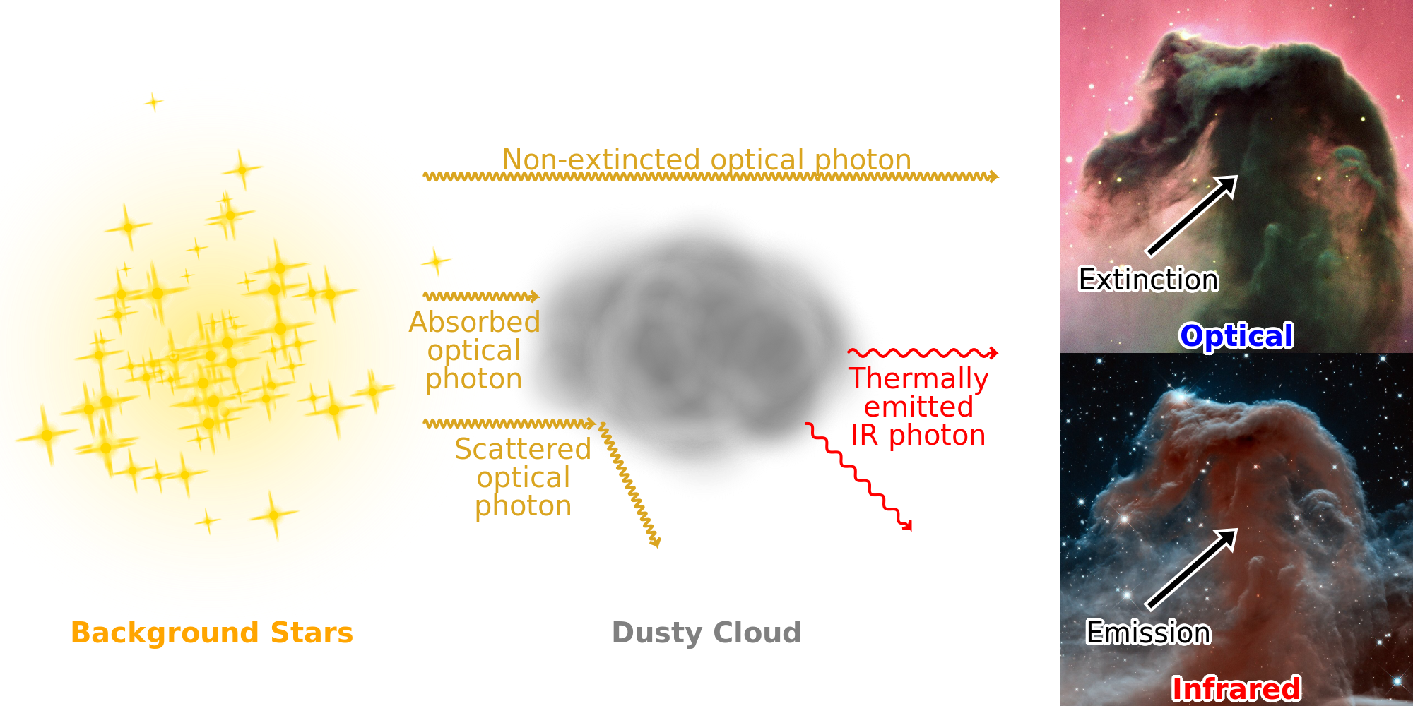
The interaction of an electromagnetic wave with dust grains results in the three following phenomena (cf. Fig. 1.11).

Absorption:: a fraction of the electromagnetic energy is stored into the grain;
Scattering:: the wave vector of the fraction that is not absorbed changes direction, its field polarization changes, but its frequency is not affected;
Emission:: the energy stored in the grain is ulteriorly re-emitted in the IR.

The sum of absorption and scattering is called extinction. These three phenomena can be modeled, assuming valence electrons are harmonic oscillators. This way, the response to an electromagnetic wave of bonds in a dielectric or free electrons in a metal can be quantified. This is illustrated in Fig. 1.12. Throughout this manuscript, we use $λ$ , $ν = c ∕ λ$ and $ω = 2 π ν$ to respectively denote the wavelength, frequency and angular frequency of an electromagnetic wave, $c$ being the speed of light (cf. Table B.2).

Figure 1.11: Absorption, scattering and emission. The images on the right are the Horsehead nebula. Licensed under CC BY-SA 4.0. Credit: Horsehead nebula images from NASA, ESA, and the Hubble Heritage Team (AURA/STScI); ESO, licensed under CC BY 4.0.

Figure 1.12: Effect of an electromagnetic wave on a dielectric. An incoming, circularly polarized, electromagnetic wave is figured in magenta. The cube on the right represents a solid. The nuclei, assumed to be fixed, are the red spheres. The valence electrons are the green ellipsoids. They are displaced out of their equilibrium positions by the electromagnetic wave, inducing a time-dependent polarization. Licensed under CC BY-SA 4.0.

1.2.1 Bonds as Harmonic Oscillators

The harmonic oscillator model is particularly useful to describe the way bonds react to electromagnetic waves.

1.2.1.1 The Harmonic Oscillator Amplitude

The position along the $x$ -axis of a unidimensional harmonic oscillator of mass, $m$ , as a function of time, $t$ , follows the equation:

\underset{inertia}{\underset{︸}{m \frac{d^{2} x (t)}{d t^{2}}}} + \underset{friction}{\underset{︸}{b \frac{d x (t)}{d t}}} + \underset{restoring force}{\underset{︸}{k_{e} x (t)}} = \underset{external force}{\underset{︸}{F (t)}},

(1.4)

where $F$ is the external force applied to the oscillator, $k_{e}$ is the strength of the restoring force, and $b$ is a dissipation constant. This equation is simply the Newton law ( $𝔽 = m ẍ$ ), where the force, $𝔽$ , has three components: (i) the external force, $F$ , displacing the oscillator out of its equilibrium position ( $x = 0$ ); (ii) the restoring force, $- k_{e} x$ , which is proportional to the distance, meaning it is stronger when the oscillator is farther away from its equilibrium position; (iii) the friction force, $- b ẋ$ , proportional to the velocity, having the effect of slowing down the oscillator.

In the case of the motion of an electron, excited by the Lorentz force of a complex, harmonic plane electromagnetic wave with angular frequency $ω$ , $F (t) = e E_{0} \exp (- i ω t)$ , Eq. ( $1.4$ ) can be rewritten:

\frac{d^{2} x (t)}{d t^{2}} + γ \frac{d x (t)}{d t} + ω_{0}^{2} x (t) = \frac{e E_{0} \exp (- i ω t)}{m_{e}},

(1.5)

where $m_{e}$ is the electron mass. We have also introduced the natural frequency, $ω_{0}$ , and the damping constant, $γ$ :

ω_{0} \equiv \sqrt{\frac{k_{e}}{m_{e}}} and γ \equiv \frac{b}{m_{e}} .

(1.6)

In this case, the restoring force is created by the atom’s electrostatic potential well, and the friction can be interpreted as collisions of the electron with the lattice. The solution to Eq. ( $1.5$ ) has the form $x (t) = x_{0} \exp (- i ω t)$ , with complex amplitude (e.g. Levi, 2016):

x_{0} = \frac{e E_{0}}{m_{e} (ω_{0}^{2} - ω^{2} - i ω γ)} .

(1.7)

It is important to consider both $\vec{x}$ and $\vec{E}$ as complex quantities, since there is a phase shift induced by the dissipation term. The module of $x_{0}$ , giving the physical value of the amplitude, is:

|x_{0}| = \frac{e | E_{0} |}{m_{e} \sqrt{{(ω^{2} - ω_{0}^{2})}^{2} + γ^{2} ω^{2}}} .

(1.8)

This is the classic harmonic oscillator solution. It is represented in Fig. 1.13. The amplitude is maximum at the resonant frequency, $ω_{r} = \sqrt{ω_{0}^{2} - γ^{2} ∕ 2}$ . If there is no dissipation ( $γ = 0$ ), the amplitude becomes infinite, and the electron escapes.

Figure 1.13: Amplitude of a forced harmonic oscillator. The left image represents the effect of an electromagnetic field, $\vec{E}$ , on an orbital. The displacement between the nucleus and the most probable position of the electron induces a permanent dipole, $\vec{p} = - e . \vec{x}$ . In this simple picture, the nucleus (cation) is assumed fixed and the electron oscillates around it. The right panel shows the amplitude of the motion of the electron (Eq. $1.8$ ) as a function of frequency, for different values of the friction, $γ$ . We have normalized both axes in order to display dimensionless quantities. Licensed under CC BY-SA 4.0.

1.2.1.2 The Plasma Frequency

Free electrons oscillate around heavy cations at the plasma frequency, $ω_{p}$ . Its formula is (cf. e.g. Chap. 1 of Krügel, 2003, for a simple proof):

ω_{p} \equiv \sqrt{\frac{n_{e} e^{2}}{m_{e} 𝜖_{0}}},

(1.9)

where $n_{e}$ is the number density of free electrons. It applies to metals, as well as actual gaseous plasmas. These media absorb and scatter electromagnetic waves with frequencies lower than $ω_{p}$ . For instance, in the case of the Earth’s ionosphere, $n_{e} ≃ 1 0^{12}$ m $^{- 3}$ , thus $ω_{p} ≃ 60$ MHz. This explains why amateur radio operators communicate over long distances at frequencies lower than this value, to benefit from the reflection of their transmission on the ionosphere (e.g. Perry et al., 2018). In the case of a metal, with density $n_{e} ≃ 1 0^{29}$ m $^{- 3}$ , $ω_{p} ≃ 20$ PHz, corresponding to a wavelength $λ_{p} ≃ 0.1 μ m$ , in the UltraViolet (UV; cf. Table A.4). This explains the shiny appearance of metals, as they are able to reflect the visible light, which has a lower frequency than UV photons. It happens that the expression of $ω_{p}$ also appears in the optical properties of dielectrics, and we will use it extensively.

1.2.1.3 The Dielectric Function

In a dielectric, an electromagnetic wave polarizes the bonds. If we consider each bond as a dipole with moment $\vec{p}$ , the polarization density is defined as:

\vec{P} = n_{e} \vec{p},

(1.10)

where $n_{e}$ is the number density of valence electrons. The induced polarization density is directly related to the electric field:

\vec{P} = 𝜖_{0} χ \vec{E},

(1.11)

where $χ$ is the electric susceptibility. The electric displacement field, $\vec{D}$ , which accounts for the charge displacement induced by an electric field $\vec{E}$ is defined as:

\vec{D} = 𝜖 \vec{E},

(1.12)

where $𝜖$ is the electric permittivity of the medium. The relative electric permittivity, $𝜖_{r}$ is defined such that: $𝜖 = 𝜖_{r} 𝜖_{0}$ . It is a macroscopic quantity, as no medium is truly continuous. At atomic scales, Eq. ( $1.12$ ) can be broken into two terms:

\vec{D} = \underset{vacuum between atoms}{\underset{︸}{𝜖_{0} \vec{E}}} + \underset{induced dipoles}{\underset{︸}{\vec{P}}} = 𝜖_{0} \underset{𝜖_{r}}{\underset{︸}{(1 + χ)}} \vec{E} .

(1.13)

The second equality derives from Eq. ( $1.11$ ). It also implies that $𝜖_{r} = 1 + χ$ . The induced polarization is, using Eq. ( $1.7$ ) and Eq. ( $1.10$ ):

\vec{P} = n_{e} e \vec{x} = \underset{𝜖_{0} χ}{\underset{︸}{\frac{n_{e} e^{2}}{m_{e}} \frac{1}{ω_{0}^{2} - ω^{2} - i ω γ}}} \vec{E} .

(1.14)

Finally, a bit of algebra and introducing the plasma frequency (Eq. $1.9$ ), gives:

𝜖_{r} (ω) = \underset{𝜖_{1} (ω)}{\underset{︸}{1 + \frac{ω_{p}^{2} (ω_{0}^{2} - ω^{2})}{{(ω_{0}^{2} - ω^{2})}^{2} + γ^{2} ω^{2}}}} + i \underset{𝜖_{2} (ω)}{\underset{︸}{\frac{ω_{p}^{2} γ ω}{{(ω_{0}^{2} - ω^{2})}^{2} + γ^{2} ω^{2}}}} .

(1.15)

This dispersion relation is called the dielectric function. It is displayed in Fig. 1.14.a. It can be related to the refractive index of the material, $m$ . Indeed, plane electromagnetic waves propagating in a dielectric have a phase velocity $v_{p h} = 1 ∕ \sqrt{𝜖 μ}$ , where $μ$ is the magnetic susceptibility (cf. e.g. Chap. 7 of Jackson, 1999, for a derivation from Maxwell’s equations). This phase velocity can also be expressed as a function of the speed of light, $c$ : $v_{p h} = c ∕ m$ , where $m$ is the refractive index. Since we can decompose $μ = μ_{r} μ_{0}$ , and because $𝜖_{0} μ_{0} = 1 ∕ c^{2}$ , we have:

m (ω) \equiv \sqrt{𝜖_{r} (ω) μ_{r} (ω)} = n (ω) + i k (ω) .

(1.16)

The refractive index is sometimes referred to as the optical constants, or simply the “ $n$ and $k$ ”. In a nonmagnetic medium, $μ_{r} = 1$ , thus:

\{\begin{matrix} 𝜖_{1} (ω) & = & n^{2} (ω) - k^{2} (ω) \\ 𝜖_{2} (ω) & = & 2 n (ω) k (ω) . \end{matrix}

(1.17)

The two complex quantities $𝜖 (ω)$ and $m (ω)$ contain the same information. Eq. ( $1.15$ ) corresponds to one single type of harmonic oscillator, that is to one mode of one type of bond. An actual dielectric is usually the linear combination of several resonances, such as Eq. ( $1.15$ ), with different sets of $ω_{p}$ , $ω_{0}$ , and $γ$ .

Figure 1.14: Idealized optical constants. Both panels show dielectric functions where the bonds (in the dielectric case) or the free electrons (in the case of a conductor) are treated as harmonic oscillators. Panel (a) displays Eq. ( $1.15$ ). We see that the imaginary part, $𝜖_{2}$ , which corresponds to the absorption, peaks around the resonant frequency and drops rapidly to zero on both sides. Panel (b) displays Eq. ( $1.28$ ). We see that the absorption by a conductor rises rapidly below the plasma frequency. It is another way to witness the fact that metals can absorb any light below $ω_{p}$ . At high frequency, $𝜖_{2} \to 0$ . Licensed under CC BY-SA 4.0.

1.2.1.4 Harmonic Oscillator Cross-Section

The flux carried by a plane electromagnetic wave is given by the time average of the Poynting vector:

⟨ | \vec{P} | ⟩ = \frac{𝜖_{0} c}{2} | \vec{E_{0}} |^{2} .

(1.18)

The power radiated by a dipole, harmonically oscillating, is (cf. e.g. Chap. 9 of Jackson, 1999):

W_{r a d} = \frac{2}{3} \frac{⟨ {\ddot{| \vec{p} |}}^{2} ⟩}{4 π 𝜖_{0} c^{3}} = \frac{ω^{4} e^{2} | x_{0} |^{2}}{12 π 𝜖_{0} c^{3}} .

(1.19)

This power is the radiation in response to the excitation by the incident wave. This is the scattering contribution. The scattering cross-section of this harmonic oscillator is thus simply: $C_{s c a} = W_{r a d} ∕ ⟨ | \vec{P} | ⟩ .$ Replacing $| x_{0} |$ by Eq. ( $1.8$ ), we obtain:

C_{s c a} (ω) = C_{T} \frac{ω^{4}}{{(ω^{2} - ω_{0}^{2})}^{2} + γ^{2} ω^{2}},

(1.20)

where we have introduced the Thomson cross-section:

C_{T} \equiv \frac{8 π}{3} {(\frac{e^{2}}{4 π 𝜖_{0} m_{e} c^{2}})}^{2} ≃ 6.66 \times 1 0^{- 29} m^{2} .

(1.21)

Now, the absorbed power comes from the dissipation into the solid. The dissipation force in Eq. ( $1.5$ ) is ${\vec{F}}_{d i s} = - m_{e} γ \dot{\vec{x}}$ . The dissipated power is thus the work of this force:

W_{d i s} = m_{e} γ | \dot{\vec{x}} |^{2} = \frac{1}{2} m_{e} γ ω^{2} | x_{0} |^{2} .

(1.22)

The absorption cross-section of the harmonic oscillator is therefore: $C_{a b s} = W_{d i s} ∕ ⟨ | \vec{P} | ⟩$ . Using Eq. ( $1.8$ ) and Eq. ( $1.21$ ), we obtain:

C_{a b s} (ω) = \frac{e^{2}}{m_{e} 𝜖_{0} c} \frac{γ ω^{2}}{{(ω^{2} + ω_{0}^{2})}^{2} + γ^{2} ω^{2}}

(1.23)

It is interesting to look at the limiting behavior of both $C_{s c a}$ and $C_{a b s}$ (see also Chap. 1 of Krügel, 2003).

At high frequency

(

ω » ω_{0}

; short wavelength), we have:

\{\begin{matrix} C_{s c a} (ω) & ≃ & C_{T} \\ C_{a b s} (ω) & ≃ & \frac{e^{2}}{4 m_{e} 𝜖_{0} c} \frac{γ}{ω^{2}} . \end{matrix}

(1.24)

Around the resonant frequency

(

ω ≃ ω_{0}

), we have:

\{\begin{matrix} C_{s c a} (ω) & ≃ & \frac{C_{T}}{4} \frac{ω_{0}^{2}}{{(ω - ω_{0})}^{2} + {(γ ∕ 2)}^{2}} \\ C_{a b s} (ω) & ≃ & \frac{e^{2}}{4 m_{e} 𝜖_{0} c} \frac{γ}{{(ω - ω_{0})}^{2} + {(γ ∕ 2)}^{2}} . \end{matrix}

(1.25)

It shows that around the resonant frequency, both $C_{s c a}$ and $C_{a b s}$ have Lorentz profiles centered at $ω_{0}$ , with Full Width at Half Maximum (FWHM), $γ$ .

At short frequency

(

ω « ω_{0}

; long wavelength):

\{\begin{matrix} C_{s c a} (ω) & ≃ & C_{T} {(\frac{ω}{ω_{0}})}^{4} \\ C_{a b s} (ω) & ≃ & \frac{e^{2} γ}{m_{e} 𝜖_{0} c ω_{0}^{2}} {(\frac{ω}{ω_{0}})}^{2} . \end{matrix}

(1.26)

Those approximations are particularly useful.

$\Rightarrow$ For dielectrics, $C_{s c a} \propto 1 ∕ λ^{4}$ and $C_{a b s} \propto 1 ∕ λ^{2}$ at long wavelength.

1.2.1.5 Optical Constants of Conductors

Eq. ( $1.15$ ) is valid for a dielectric, as it assumes the medium is only constituted of dipoles. This is not the case in a conductor where there are also free charges. An electromagnetic wave induces a current, $\vec{j}$ , related to the electric field, $\vec{E}$ , by the conductivity, $σ$ :

\vec{j} = σ \vec{E} = n_{e} e \vec{v},

(1.27)

where the second equality relates the current to its microscopic origin, the velocity of free electrons, $\vec{v}$ . Maxwell’s equations for plane waves give (e.g. Chap. 7 of Jackson, 1999):

𝜖_{r} (ω) = \underset{bound electrons}{\underset{︸}{𝜖_{d} (ω)}} + \underset{free electrons}{\underset{︸}{i \frac{σ (ω)}{𝜖_{0} ω}}},

(1.28)

where $𝜖_{d} (ω)$ is the leftover dielectric term. We can apply the harmonic oscillator model again to these free electrons. The difference is that there is no restoring force, $ω_{0} = 0$ . From Eq. ( $1.7$ ), the velocity of free electrons becomes:

|\vec{v}| = \frac{e | \vec{E} |}{m_{e} (γ - i ω)} .

(1.29)

Injecting this quantity in Eq. ( $1.27$ ), we obtain:

σ (ω) = 𝜖_{0} ω_{p}^{2} \frac{γ}{γ^{2} + ω^{2}} + i 𝜖_{0} ω_{p}^{2} \frac{ω}{γ^{2} + ω^{2}} .

(1.30)

Focussing on the free electron term in Eq. ( $1.28$ ), i.e. assuming $𝜖_{d} = 0$ , we get:

𝜖_{r} (ω) = \underset{𝜖_{1} (ω)}{\underset{︸}{1 - \frac{ω_{p}^{2}}{γ^{2} + ω^{2}}}} + i \underset{𝜖_{2} (ω)}{\underset{︸}{\frac{γ}{ω} \frac{ω_{p}^{2}}{γ^{2} + ω^{2}}}} .

(1.31)

It is also known as the Drude model. This equation is displayed in Fig. 1.14.b. Interestingly enough, the cross-sections of Eq. ( $1.20$ ) and Eq. ( $1.23$ ) apply also to conductors, with $ω_{0} = 0$ . We can easily derive their limiting behavior.

$\Rightarrow$ Conductors have the same behavior than dielectrics at long wavelength: $C_{s c a} \propto 1 ∕ λ^{4}$ and $C_{a b s} \propto 1 ∕ λ^{2}$ .

1.2.1.6 The Kramers-Kronig Relations

The residue theorem implies that, if $f (x)$ is a complex function of the complex variable $x$ , analytical over $ℑ (x) \geq 0$ , and dropping faster than $1 ∕ | x |$ , we have the relation:

f (ω) = \frac{1}{i π} P \int_{- \infty}^{\infty} \frac{f (x)}{x - ω} d x,

(1.32)

with $ω$ real and positive. We have used the Cauchy principal value:

P \int_{- \infty}^{\infty} \frac{f (x)}{x - ω} d x = \lim_{δ \to 0} (\int_{- \infty}^{ω - δ} \frac{f (x)}{x - ω} d x + \int_{ω + δ}^{\infty} \frac{f (x)}{x - ω} d x),

(1.33)

which is simply an integral avoiding the singularity in $x = ω$ . Decomposing $f (x) = f_{1} (x) + i f_{2} (x)$ , we obtain cross-relations between $f_{1} (x)$ and $f_{2} (x)$ . These general mathematical relations are usually applied to the susceptibility, from which we derive the dielectric function (e.g. Chap. 21 of Draine, 2011):

\{\begin{matrix} 𝜖_{1} (ω) - 1 & = & \frac{2}{π} P \int_{0}^{\infty} \frac{x 𝜖_{2} (x)}{x^{2} - ω^{2}} d x \\ 𝜖_{2} (ω) & = & - \frac{2}{π} ω P \int_{0}^{\infty} \frac{𝜖_{1} (x) - 1}{x^{2} - ω^{2}} d x . \end{matrix}

(1.34)

These relations are known as the Kramers-Kronig relations.

Implications. We only need to specify $𝜖_{1}$ or $𝜖_{2}$ at all frequencies, and can use Eq. ( $1.34$ ) to derive the other one. These relations are used to check laboratory data consistency (e.g. Zubko et al., 1996).

Interpretation. They are a consequence of the causality requirement for a linear system (here, we have $\vec{P} = 𝜖_{0} χ \vec{E}$ ). In our case, they impose that the response of the polarization does not precede the effect of the electric field. Sect. 62 of Landau & Lifshtiz (1960), Chap. 21 of Draine (2011), and Chap. 2 of Krügel (2003) discuss these relations more extensively.

Constraint on the Cross-Section. They give some constraints on the long wavelength behavior of the dielectric function. Let’s assume that $𝜖_{2} (ω) \propto ω^{β - 1}$ for $ω < δ$ , for an arbitrary $δ$ . The first relation tells us that:

𝜖_{1} (0) = 1 + \frac{2}{π} \int_{0}^{δ} x^{β - 2} d x + \int_{δ}^{\infty} \frac{𝜖_{2} (x)}{x} d x .

(1.35)

The second integral is finite by requirement. For the first integral to be finite, we need to have $β > 1$ . At long wavelength, Eq. ( $1.15$ ) tells us that, for a dielectric:

\{\begin{matrix} 𝜖_{1} (ω) & \underset{ω \to 0}{\to} & 1 + {(\frac{ω_{p}}{ω_{0}})}^{2} & = & const \\ 𝜖_{2} (ω) & \underset{ω \to 0}{\to} & \frac{ω_{p}^{2} γ}{ω_{0}^{4}} ω & « & 𝜖_{1} (ω) . \end{matrix}

(1.36)

We will see in Eq. ( $1.45$ ) that, at long wavelength, $C_{a b s} \propto 𝜖_{2} ∕ [{(𝜖_{1} + 2)}^{2} + 𝜖_{2}^{2}] ∕ λ$ . Using Eq. ( $1.36$ ), we get $C_{a b s} (λ) \propto 𝜖_{2} (λ) ∕ λ \propto λ^{- β}$ . We will see in Sect. 3.1.2 that this $β$ parameter is sometimes referred to as the emissivity index.

$\Rightarrow$ Assuming that $C_{a b s} (λ) \propto λ^{- β}$ at long wavelengths, we need to have $β > 1$ .

1.2.2 Grain Optical Properties

1.2.2.1 Why Are Most Dust Features in the MIR?

Figure 1.15: Molecular transitions. The different types of transitions are illustrated with the CO molecule. Licensed under CC BY-SA 4.0.

All but one spectral features of the interstellar grain candidates we have listed in Table 1.3 are in the MIR. This is a general trend (e.g. Table 1 of van der Tak et al., 2018). It can be understood by making an analogy with the different types of molecular transitions (cf. e.g. Chap. 2 of Tielens, 2005, for a review). Those are illustrated in Fig. 1.15.

Electronic transitions: are transitions between the quantum harmonic oscillator levels of the bonding electron. In the case of solids, they are transitions between bands, such as the $π \to π^{⋆}$ transition of aromatic carbon, at 2175 Å (cf. Sect. 1.1.4). The natural frequency of these resonances is given by Eq. ( $1.6$ ): $ω_{0} = \sqrt{k_{e} ∕ m_{e}}$ . The energy of these resonances is comparable to the binding energy, or the band gap. They typically range between $≃ 4$ and $≃ 20$ eV. They are thus in the UV domain ( $λ ≃ 0.06 - 0.30 μ m$ ).
Vibrational transitions: are associated with the stretching or bending of a bond. These modes involve the motion of the nuclei, which are much heavier than the electrons. Their frequency is $ω_{v} = \sqrt{k_{v} ∕ μ_{1, 2}}$ , where $μ_{1, 2} = m_{1} m_{2} ∕ (m_{1} + m_{2})$ is the reduced mass of the two atoms, $m_{1}$ and $m_{2}$ . Typically, $μ_{1, 2} = 0.9, 6, 10 \times m_{p}$ for C–H, C–C and Si–O bonds, respectively ( $m_{p}$ is the proton mass; cf. Table B.2). At first order, the new force constant is similar to previously, $k_{e} ≃ k_{v}$ . The frequency is now reduced by a factor $≃ \sqrt{m_{e} ∕ μ_{1, 2}} ≃ 0.007 - 0.02$ . These transitions are thus in the MIR ( $λ ≃ 2 - 40 μ m$ ). They are the most relevant transitions for ISD.
Rotational transitions: are associated with the rotation of the molecule. Their energy depends on the centrifugal force, which reduces the frequency by a factor $≃ m_{e} ∕ m_{p}$ . These transitions are thus in the millimeter regime. Most dust grains do not have detectable rotational transitions, because of their inertia. Only the smallest grains have a non-negligible rotational emission that will be discussed in Sect. 2.2.2.3.

1.2.2.2 Dielectric Functions of Realistic Materials

The dielectric functions of Eq. ( $1.15$ ) and Eq. ( $1.28$ ) correspond to simple cases where there is only one type of oscillator. Realistic materials have more complex structures, with several modes per bond. Deriving dielectric functions of potential interstellar grain analogs is the subject of a rich literature. There are three types of approaches to determine the dispersion relation of a medium.

The theoretical knowledge: of the microscopic structure of the crystal can be used to determine the different resonances that we have demonstrated in Sect. 1.2.1. The resonant or plasma frequency, as well as the collisional rates ( $γ$ ) have to be known. The Kramers-Kronig relations (Sect. 1.2.1.6) can be used to obtain complementary constraints.
Laboratory data: about the spectral profile of some features, or the density of the material, or any relevant characteristics can also be used. The ISM community is active in this field, as our results largely depend on the accurate values of atomic and molecular data. Several teams focus their research effort on laboratory measures of dust analogs.
Astronomical observations: can be used to constrain some features. The most famous example is the use of observations of the 9.7 and 18 $μ m$ band profiles to build the optical properties of astronomical silicates, by Draine & Lee (1984). Indeed, we have seen in Sect. 1.1.4 that there is a diversity of silicate composition, and we do not know which one is relevant to ISD (it is likely a mixture).

These approaches are not exclusive and are usually combined as observations and laboratory data are always partial. The work by Draine & Lee (1984) was the first study to use these principles to derive the UV-to-mm dielectric functions of graphite and astronomical silicates. We now have a better knowledge of the dispersion relations of several important materials: (i) silicates (e.g. Laor & Draine, 1993; Weingartner & Draine, 2001a; Draine, 2003b,c); (ii) amorphous carbon (e.g. Rouleau & Martin, 1991; Zubko et al., 1996; Jones, 2012a,b,c); (iii) graphite (e.g. Laor & Draine, 1993; Draine, 2003b,c, 2016); (iv) PAHs (e.g. Li & Draine, 2001; Draine & Li, 2007); and (v) composite grains (e.g. Köhler et al., 2014, 2015). Fig. 1.16 shows a few examples.

Figure 1.16: Dielectric functions of different materials. In each panel, we show the real part of the dielectric function as $𝜖_{1} - 1$ (blue) and $1 - 𝜖_{1}$ (green), as this quantity can be negative. The imaginary part, $𝜖_{2}$ , is in red. Panel (a) shows the astronomical silicates by Draine (2003b,c). Panel (b) shows the ACAR type of amorphous carbon by Zubko et al. (1996). These are produced by arc discharges between amorphous carbon electrodes in a 10 mbar Ar atmosphere. Panel (c) and (d) show the graphite by Draine (2003b,c). Graphite is anisotropic, as we have seen in Fig. 1.9.e. It is usually approximated by mixing 2/3 of the optical properties parallel to the graphene sheets (c), and 1/3 perpendicular (d). Licensed under CC BY-SA 4.0.

1.2.2.3 Computing Grain Cross-Sections

The dielectric functions are intensive quantities characterizing the bulk optical properties of solids, but independent of their size and shape. To compute usable absorption and scattering cross-sections, there is one last step to do. Let’s assume our grains are spheres of radius $a$ .

The extinction cross-section of the grain can be written:

C_{e x t} (λ, a) = \underset{geometric cross-section}{\underset{︸}{π a^{2}}} \times \underset{efficiency}{\underset{︸}{Q_{e x t} (λ, a)}} .

(1.37)

This expression is simply the geometric cross-section, $π a^{2}$ , times an extinction efficiency, $Q_{e x t}$ , which is a dimensionless quantity. We can express the scattering and absorption cross-section the same way:

\{\begin{matrix} C_{s c a} (λ, a) & = & π a^{2} Q_{s c a} (λ, a) \\ C_{a b s} (λ, a) & = & π a^{2} Q_{a b s} (λ, a) . \end{matrix}

(1.38)

Out of these three efficiencies, only two are independent, as we have $Q_{e x t} = Q_{s c a} + Q_{a b s}$ .

Another useful quantity that can be derived from the efficiencies is the albedo, quantifying the fraction of the incident light that is scattered by the grain:
$\tilde{ω} (λ, a) \equiv \frac{C_{s c a} (λ, a)}{C_{e x t} (λ, a)} = \frac{Q_{s c a} (λ, a)}{Q_{e x t} (λ, a)} .$ (1.39)

Let’s call

𝜃

the angle between the directions of the incident and scattered light. The probability distribution of scattering angles is called the scattering phase function:

Φ (\cos 𝜃, λ, a) \equiv \frac{1}{C_{s c a} (λ, a)} \frac{d C_{s c a} (\cos 𝜃, λ, a)}{d Ω},

(1.40)

where $C_{s c a} (\cos 𝜃, λ, a)$ is the differential scattering cross-section (i.e. the cross-section for scattering in a given direction), and $d Ω = d \cos 𝜃 d ϕ$ is the solid angle element. It is normalized over all directions, such that:

\iint_{Ω} Φ (\cos 𝜃, λ, a) d Ω = 2 π \int_{- 1}^{1} Φ (\cos 𝜃, λ, a) d \cos 𝜃 = 1 .

(1.41)

For isotropic scattering, we have $Φ (\cos 𝜃, λ, a) = 1 ∕ 4 π$ . The first moment of this distribution is called the asymmetry parameter, defined as:

g (λ, a) = ⟨ \cos 𝜃 ⟩ = 2 π \int_{- 1}^{1} Φ (\cos 𝜃, λ, a) \cos 𝜃 d \cos 𝜃 .

(1.42)

This parameter is a direct product of Mie theory. Forward and backward scattering correspond to $⟨ \cos 𝜃 ⟩ ≃ 1$ and $⟨ \cos 𝜃 ⟩ ≃ - 1$ , respectively, whereas isotropic scatterers have $⟨ \cos 𝜃 ⟩ ≃ 0$ . There are approximate analytical phase functions. The most famous is from Henyey & Greenstein (1941):

Φ (\cos 𝜃, λ, a) = \frac{1}{4 π} \frac{1 - g^{2} (λ, a)}{{(1 + g^{2} (λ, a) - 2 g (λ, a) \cos 𝜃)}^{3 ∕ 2}} .

(1.43)

Other distributions have been proposed (e.g. Draine, 2003b).

The treatment to compute $Q_{s c a}$ , $Q_{a b s}$ and $g$ depends on the value of the size parameter:

x = \frac{2 π a}{λ} .

(1.44)

As long as we do not zoom in scales where the hypothesis of a continuous medium breaks down, that is scales of a few Å (i.e. grains made of a few atoms, or hard X-ray photons), the estimation of the efficiencies of a grain only depends on $x$ and $m$ . The Mie theory (cf. e.g. Chap. 4 of Bohren & Huffman, 1983) ⁵ is the central tool to compute grain cross-sections. It is a numerical method, exactly solving Maxwell’s equations for the scattering of a plane electromagnetic wave by a homogeneous sphere of known refractive index, $m (λ)$ . Several regimes can be identified, depending on the value of the size parameter. They are illustrated in Fig. 1.18. In Fig. 1.19, we show the actual cross-sections of silicate and graphite grains of different sizes.

Geometrical optics. It is the regime for which $x » 1$ (cf. e.g. Chap. 7 of Bohren & Huffman, 1983). For interstellar grains, which have submicronic sizes, it corresponds to UV wavelengths and shorter. This regime is more relevant to circumstellar dust, where grains can be significantly larger. In geometrical optics, the undulatory nature of light is put aside. Instead, light is modeled as rays, using the formalism of Fresnel. Mie theory is valid in this regime, but numerical problems start arising.

The important feature of this regime is that, $Q_{s c a} ≃ Q_{a b s} ≃ 1$ (cf. Fig. 1.18.b). This can also be seen in panels (a) to (d) of Fig. 1.19. When the size of the grain increases, the range where both $Q_{s c a}$ and $Q_{a b s}$ are flat extends to shorter wavelengths. The cross-sections are independent of wavelength, as the grains are effectively behaving as opaque circular screens. It also means that the cross-section is proportional to the area of the grain, but independent of its volume.
$Q_{s c a} ≃ Q_{a b s} ≃ 1$ implies that $Q_{e x t} ≃ 2$ , meaning that the extinction cross-section is twice the geometric cross-section. This counter-intuitive result is called the extinction paradox (Chap. 4 of Bohren & Huffman, 1983, for an extensive discussion). It is a real diffraction effect, that is not actually predicted by the methods of geometrical optics, for which $Q_{e x t} ≃ 1$ . Its resolution lies in accounting for the diffraction around the grain. It is illustrated in Fig. 1.17. The exact interpretation of this paradox is still debated nowadays (e.g. Berg et al., 2011).
Another feature of this regime is that grains are efficient forward scatterers ( $⟨ \cos 𝜃 ⟩ ≃ 1$ ; Fig. 1.18.c).

Figure 1.17: Illustration of the extinction paradox. We have represented two situations. In panel (a), we show the radiation from a distant star passing through a circular pupil of radius $a$ , and projected onto the plane of a detector. We assume that: (i) the star is very distant, so that the incident wave can be considered planar; (ii) the detector is at a distant from the pupil much larger than $a$ . The observed pattern is a series of Airy rings. In panel (b), we show the same stellar radiation absorbed and scattered by a dust grain of the same radius $a$ as the pupil, at the same distance from a detector. The observed pattern is made of the same Airy rings, but there is a bright spot in the center. This property is a result of Babinet’s theorem. This theorem is based on the fact that the wave function of a plane wave, $ψ (x, y)$ , diffracted by a pupil of transmission $T (x, y)$ , is proportional to the Fourier transform of the pupil, $F (T)$ . Here, the direction represented by the blue arrow is the $z$ axis. The $x$ and $y$ axes are the coordinates in the plane of the pupil and of the detector, both being parallel. If we have two pupils, $T_{(a)}$ and $T_{(b)}$ , that are complementary, that is $T_{(a)} (x, y) + T_{(b)} (x, y) = 1$ , $\forall (x, y)$ , we have, by linearity of the Fourier transform $ψ_{(a)} (x, y) + ψ_{(b)} (x, y) \propto F (T_{(a)}) + F (T_{(b)}) = δ (x, y)$ , where $δ$ is the Dirac distribution centered in the middle of the screen. In our case, the two complementary pupils are the circular hole in panel (a), and the grain, appearing as a circular screen to the stellar radiation, in panel (b). The intensity is the squared module of the wave function, $I (x, y) = | ψ (x, y) |^{2}$ . We see that $ψ_{(b)} (x, y) = ψ_{0} δ (x, y) - ψ_{(a)} (x, y)$ , thus $I_{(b)} (x, y) = I_{spot} δ (x, y) + I_{(a)} (x, y)$ , confirming that the pattern in panel (b) is the pattern in panel (a) plus a bright spot. In panel (b), the bright spot is just the incident wave (rays parallel to the $z$ axis). We note that $I_{(a)} (x, y) = I_{(b)} (x, y)$ , except in $(0, 0)$ . The incident light of intensity $I_{0}$ on the grain surface ( $π a^{2}$ ) is absorbed. Thus, the absorbed power is $P_{a b s} = π a^{2} I_{0}$ . Now, the Airy pattern is the fraction diffracted by the grain contour, that is the scattered light. Babinet’s theorem tells us that it is identical in both cases we have represented. We clearly see in panel (a) that the scattered power is also $P_{s c a} = π a^{2} I_{0}$ . The grain thus extinct a power $P_{e x t} = 2 π a^{2} I_{0}$ . This is the extinction paradox: (i) the flux incident on the grain surface is fully absorbed; (ii) the contour of the grain scatters the same power at small angles, corresponding to the Airy rings in both panels. Licensed under CC BY-SA 4.0.

The Mie regime. It corresponds to grain sizes comparable to the wavelength of the incident light ( $x ≃ 1$ ). Mie theory is valid outside this regime, but this is the regime where none of the other approximations are valid.

The optical properties have non-trivial features, depending on $x$ and on the actual resonances of $m$ . For instance, panels (a) and (c) of Fig. 1.19 show the 9.7 and 18 $μ m$ features of silicates. These features disappear only for radii $a ≳ 10$ $μ m$ , as the geometrical optics regime extends in the mid-IR (MIR; cf. Table A.4), in this case.
The scattering pattern is non-trivial, $⟨ \cos 𝜃 ⟩$ varying between 0 and 1. It is schematically represented in the central cartoon at the top of Fig. 1.18, using the Eq. ( $1.43$ ). It shows that backward scattering is likely, although forward scattering is more probable.
Finally, we notice small oscillations in the visible and near-IR (NIR; cf. Table A.4) ranges, mostly visible in the $Q_{a b s}$ of micronic size grains (panels (c) and (d) of Fig. 1.19). These patterns are called interference structure. They are due to the interference between the incident and scattered waves. They are more prominent for weakly absorbent material, such as silicate, which is more transparent than graphite (cf. Sect. 1.1.4).

Figure 1.18: Mie, Rayleigh and geometric optics regimes. The top pictures represent the scattering pattern (in magenta) of a spherical grain (red sphere), in the three regimes. The direction of the incident photon is shown in yellow. The scattering pattern has been calculated using the Henyey & Greenstein (1941) phase function. The length of each wiggly arrow is proportional to its scattering probability. The three panels plot below show the optical properties of a $a = 0.1$ $μ m$ radius silicate, by Draine (2003b,c). Licensed under CC BY-SA 4.0.

Figure 1.19: Cross-sections of silicate and graphite grains. The color lines show the optical properties of grains with different radius, $a$ , from Draine (2003b,c). Licensed under CC BY-SA 4.0.

The Rayleigh regime. It corresponds to grain sizes significantly smaller than the wavelength of the incident light, $x « 1$ (cf. e.g. Chap. 5 of Bohren & Huffman, 1983). In the case of interstellar grains, it applies essentially to the NIR regime and longward. The refraction index needs to be small, too: $| m | x « 1$ . The solutions are analytic (e.g. Li, 2008):

\{\begin{matrix} C_{s c a} (λ, a) & = & \frac{128 π^{5}}{3} {|\frac{𝜖_{r} (λ) - 1}{𝜖_{r} (λ) + 2}|}^{2} \frac{a^{6}}{λ^{4}} \\ C_{a b s} (λ, a) & = & 24 π^{2} \frac{𝜖_{2} (λ)}{{(𝜖_{1} (λ) + 2)}^{2} + 𝜖_{2}^{2} (λ)} \frac{a^{3}}{λ} . \end{matrix}

(1.45)

Eq. ( $1.45$ ) and panels (a) to (d) of Fig. 1.19 show that $Q_{s c a} ∕ a^{4}$ and $Q_{a b s} ∕ a$ are independent of radius in this regime. This explains why small grains have a negligible albedo, whereas large grains are efficient scatterers.
The fact that $Q_{a b s} ∕ a$ is independent of radius implies that the absorption cross-section is proportional to the grain volume: $C_{a b s} \propto a^{3}$ . The dust mass can thus be probed by measures in absorption or in emission. An interpretation of this property is that, the wavelength being comparable to the size of the grain, each bond can interact with the electromagnetic field, independently of its location within the solid. The interaction of the incident light with the grain is thus proportional to the total number of oscillators, which is proportional to the mass.
It explains why scattering appears negligible in this regime: $(C_{s c a} \propto a^{6}) « (C_{a b s} \propto a^{3})$ . Finally, we can see that scattering is isotropic ( $⟨ \cos 𝜃 ⟩ ≃ 0$ ).

$\Rightarrow$ The absorption cross-section of most interstellar grains, in the NIR-to-mm window, is proportional to their volume. The dust mass can thus be probed by absorption or emission measures.

1.2.2.4 Beyond Homogeneous Spheres

Mie theory is restricted to homogeneous spheres. However, there are several observational indications that this hypothesis is not fully accurate (cf. Sect. 4.2.1.1).

Grains are rapidly formed and destroyed in the ISM, implying that they likely are composites of several materials with different dielectric functions, and voids.
The polarization of starlight and of ISM emission in the far-IR (FIR; cf. Table A.4) indicates that at least some of the grains are elongated.

There are several methods to estimate cross-sections of grains beyond the hypothesis of homogeneous spheres.

Effective medium theory (EMT). EMT is a class of methods to replace the individual dielectric functions of a composite material by an average, $𝜖_{av} (λ)$ . Cross-sections can then be estimated using Mie theory or any other approximation. EMT assumes that the different domains are smaller than the wavelength and well-mixed in the grain. There are different mixing rules (cf. e.g. Chap. 8 of Bohren & Huffman, 1983). It seems that their accuracy depends on the type of sample they are applied to, as independent studies find better agreements with one or the other (e.g. Abeles & Gittleman, 1976; Perrin & Lamy, 1990).

Maxwell Garnett’s rule

assumes that the medium is constituted of a matrix with dielectric function

𝜖_{m} (λ)

, and some inclusions. The inclusions can be of

N

different types, with dielectric functions

𝜖_{i} (λ)

(

i = 1 \dots N

), and volume filling factors,

ϕ_{i}

. It is implicit that

ϕ_{i} « 1

𝜖_{av} (λ) = \frac{𝜖_{m} (λ) + \sum_{i = 1}^{N} ϕ_{i} c_{i} 𝜖_{i} (λ)}{1 + \sum_{i = 1}^{N} ϕ_{i} c_{i}},

(1.46)

with:

c_{i} = \frac{3 𝜖_{m} (λ)}{𝜖_{i} (λ) + 2 𝜖_{m} (λ)} .

(1.47)

Bruggeman’s rule

does not put a hierarchy between a predominant matrix and a few inclusions. The dielectric function is the solution of:

\sum_{i = 1}^{N} ϕ_{i} \frac{𝜖_{i} (λ) - 𝜖_{av} (λ)}{𝜖_{i} (λ) + 2 𝜖_{av} (λ)} = 0 .

(1.48)

Ellipsoids in the Rayleigh regime. They have general analytical solutions (e.g. Chap. 5 of Bohren & Huffman, 1983). When the three axes of the ellipsoid are aligned on the coordinates $x, y, z$ and if the the electric field is along $x$ , we have:

\{\begin{matrix} C_{s c a} (λ, a) & = & \frac{128 π^{5}}{27} {|\frac{𝜖_{r} (λ) - 1}{1 + (𝜖_{r} (λ) - 1) L_{x}}|}^{2} \frac{a^{6}}{λ^{4}} \\ C_{a b s} (λ, a) & = & \frac{8 π^{2}}{3} ℑ [\frac{𝜖_{r} (λ) - 1}{1 + (𝜖_{r} (λ) - 1) L_{x}}] \frac{a^{3}}{λ}, \end{matrix}

(1.49)

where $L_{x}$ is the shape factor. Noting $l_{a} > l_{b}$ the two lengths, oblate spheroids have dimensions along the three axes $(l_{a}, l_{a}, l_{b})$ , whereas prolate spheroids have dimensions $(l_{a}, l_{b}, l_{b})$ (cf. Fig. 1.20). With these notations, the shape factor is (e.g. Chap. 22 of Draine, 2011):

\{\begin{matrix} L_{x} & = & \frac{1 + ξ^{2}}{ξ^{2}} [1 - \frac{\arctan ξ}{ξ}] & for oblate spheroids \\ L_{x} & = & \frac{1 - ξ^{2}}{ξ^{2}} [\frac{1}{2 ξ} \ln (\frac{1 + ξ}{1 - ξ}) - 1] & for prolate spheroids, \end{matrix}

(1.50)

with $ξ^{2} = | 1 - {(l_{b} ∕ l_{a})}^{2} |$ . In case of randomly oriented ellipsoids, we simply need to take the arithmetic mean of the cross-sections along the three axes.

Figure 1.20: Oblate and prolate spheroids. Credit: volumes produced with Mathematica.

Discrete Dipole Approximation (DDA). DDA (Purcell & Pennypacker, 1973) ⁶ allows the user to model complex composite grains as arbitrary arrays of independent domains. These domains are approximated by a series of discrete dipoles, which must be much smaller than the incoming wavelength. This method is computer intensive, but very flexible (cf. e.g. the results of Köhler et al., 2015; Ysard et al., 2018). We show some of the results of Köhler et al. (2015) in Fig. 1.21. This figure exhibits an important result we will discuss later:

$\Rightarrow$ the addition of mantles and the aggregation of grains tend to increase the absorptivity per unit mass in the FIR window.

Figure 1.21: Absorption cross-sections of grain aggregates computed with DDA. The curves in the left panel are the absorption cross-sections of grains of radius $a = 0.2$ $μ m$ : $C_{a b s} (a, λ) ∕ m (a) = 3 ∕ (4 ρ) \times Q_{a b s} (a, λ) ∕ a$ , where $ρ$ is the density. The four curves correspond to the four main mixtures of the THEMIS model (Jones et al., 2013, 2017), represented in the right panel: (i) the Core-Mantle (CM) mixture is made amorphous Forsterite and Enstatite with Fe and FeS (troilite) inclusions, and aliphatic amorphous carbon (a-C:H); both grains are coated with an aromatic mantle (a-C); (ii) the Core-Mantle-Mantle (CMM) is the CM mixture with additional coating by aliphatic material; (iii) the Aggregate-Mantle-Mantle (AMM) mixture is constituted of aggregated CMM grains; (iv) the Aggregate-Mantle-Mantle-Ice (AMMI) mixture is the AMM aggregates coated with water ice. The CM optical properties are from Jones et al. (2013). The CMM, AMM and AMMI optical properties have estimated by Köhler et al. (2015) using DDA. Notice the apparition of the 3 $μ m$ water ice band (Fig. 2.12) in the AMMI model. Licensed under CC BY-SA 4.0.

1.2.2.5 Polarization

The real part of the electric field of a monochromatic, plane electromagnetic wave, propagating along the $z$ -axis, can be written at time $t$ and at $z = 0$ :

ℜ (\vec{E}) = \vec{E_{1}} \cos ω t + \vec{E_{2}} \sin ω t,

(1.51)

where $\vec{E_{1}} ⊥ \vec{E_{2}}$ (cf. e.g. Chap. 2 of Bohren & Huffman, 1983). This is the parametric equation of an ellipse in the $(x, y)$ plane (cf. Fig. 1.22.a). It is the most general case, called elliptical polarization. It is fully characterized by the modules of $\vec{E_{1}}$ and $\vec{E_{2}}$ , the angle $φ$ and the rotation direction $η = \pm 1$ (-1: clockwise; +1:counterclockwise). Particular cases are: (i) linear polarization, if $| \vec{E_{1}} | = 0$ or $| \vec{E_{2}} | = 0$ ; and (ii) circular polarization, if $| \vec{E_{1}} | = | \vec{E_{2}} |$ .

Figure 1.22: Stokes parameters. Panel (a) displays the notations we have used to parametrize the elliptical polarization. Panels (b) to (g) demonstrate the type of polarization each parameter represents (linear or circular, in different directions), when the rest is zero. Licensed under CC BY-SA 4.0.

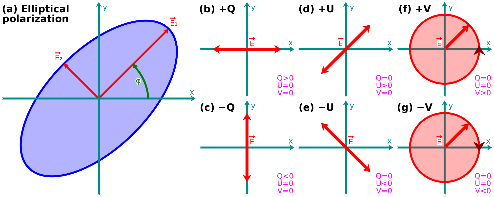
The Stokes parameters. They constitute a four element vector easier to observationally measure than the ellipse parameters. They are noted $(I, Q, U, V) = \vec{S}$ . $I$ is the total intensity of the beam, that can be partially polarized. The three others can be expressed as:

\{\begin{matrix} Q & = & (| \vec{E_{1}} |^{2} - | \vec{E_{2}} |^{2}) \cos (2 φ) \\ U & = & (| \vec{E_{1}} |^{2} - | \vec{E_{2}} |^{2}) \sin (2 φ) \\ V & = & 2 η | \vec{E_{1}} | | \vec{E_{2}} | . \end{matrix}

(1.52)

The interpretation of these parameters is illustrated in Fig. 1.22. They allow us to decompose the light into its linear and circular polarization components. The intensity of the polarized light is $I_{p} = \sqrt{Q^{2} + U^{2} + V^{2}} \leq I$ . It is also frequent to quote the linearly polarized intensity:

P \equiv \sqrt{Q^{2} + U^{2}},

(1.53)

and the linear polarization fraction, $P ∕ I$ .

Grain alignment. Asymmetric grains tend to be aligned with the magnetic field. If we consider the simple case of spheroidal grains (cf. Fig. 1.20): (i) the rotation axis of oblate grains is along their symmetry axis; (ii) the rotation axis of prolate grains is perpendicular to their long axis, their cross-section thus needs to be integrated over their spinning dynamics (e.g. Guillet et al., 2018). The rotation axis of the grains tends to align with the magnetic field, $\vec{B}$ . This is represented in panels (b) and (c) of Fig. 1.23. Several mechanisms have been proposed to explain this alignment (cf. Andersson et al., 2015, for a review). Nowadays, Radiative Alignment Torques (RAT; Dolginov & Mitrofanov, 1976) are favored, because they provide the best account of the observational constraints. This complex scenario is based on the fact that irregular grains have different cross-sections for clockwise and counterclockwise circularly polarized light. Light scattering on such grains therefore provides a torque that increases the angular momentum of the grains. If these grains have paramagnetic inclusions (such as iron), the grain rotation precesses and aligns with $\vec{B}$ . Although the alignment is caused by the radiation field, it is independent of its direction. This mechanism becomes inefficient at high optical depth, which is consistent with observations.

Polarization by scattering. It is represented on Fig. 1.23.a. When an incident beam is scattered by a grain (this grain does not have to be asymmetric), the electric field component in the scattering plane is diminished, inducing a polarization perpendicular to the plane. The larger the scattering angle is, the larger the polarization. The polarization of an incident Stokes vector, $\vec{S_{i}}$ , resulting in a scattered beam, $\vec{S_{s}}$ , is described as: $\vec{S_{s}} = \overset{⃡}{M} \vec{S_{i}}$ , where $\overset{⃡}{M}$ is the $4 \times 4$ Müller matrix (cf. Chap. 3 of Bohren & Huffman, 1983, for different examples of Müller matrices). This polarization process is not related to grain alignment with the magnetic field, but it depends on the distribution of stars and dust clouds (e.g. Wood, 1997).

Dichroic extinction. It is the selective extinction of the electric field oscillating along the major axis of an elongated grains. It is represented in Fig. 1.23.b. Since grains in the diffuse ISM tend to align their rotation axis with the magnetic field, they polarize starlight parallel to $\vec{B}$ . For this reason, the polarization of starlight has historically been used to map the magnetic field of the MW (Mathewson & Ford, 1970).

Polarized emission. The polarization of the emission by elongated grains has been predicted by Stein (1966). Such grains emit IR light preferentially polarized along the direction of their major axis. Since their major axis is perpendicular to the magnetic field, their IR emission is perpendicular to $\vec{B}$ . It is represented in Fig. 1.23.c. The FIR polarized emission has been extensively used to map the magnetic field in the MW, with the Planck satellite (e.g. Planck Collaboration et al., 2016d).

$\Rightarrow$ Grain polarization is parallel to the magnetic field in the visible and perpendicular in the IR: $\vec{P_{v i s}} ∥ \vec{B}$ and $\vec{P_{I R}} ⊥ \vec{B}$ .

Figure 1.23: The three types of grain-induced polarization of light. Panel (a) represents the unpolarized starlight radiation being scattered by a grain. The electric field of the scattered light oscillates predominantly perpendicularly to the scattering plane. The larger the scattering angle is, the higher the linear polarization fraction is. Panels (b) and (c) represent a single prolate grain whose rotation axis is aligned with the magnetic field, $\vec{B}$ . The case of oblate grains is more trivial as their rotation axis is their symmetry axis. Panel (b) illustrates dichroic extinction of starlight in the visible/near-IR. The grain extinct preferentially the component of the electric field oscillating in its rotation plane. The extincted starlight is thus polarized parallel to $\vec{B}$ . Panel (c) shows the IR emission of the same prolate grain is polarized along its major axis, perpendicular to $\vec{B}$ . In both panels (b) and (c), we have represented the optimal case, when the magnetic field is perpendicular to the sightline. In the more general case, the polarization will be relative to the projection of $\vec{B}$ on the plane of the sky. Licensed under CC BY-SA 4.0.

1.2.3 Heat Capacities

In Sect. 1.2.1, presenting the harmonic oscillations of valence electrons, we argued that the energy dissipation was due to collisions with the lattice. The energy absorbed by the grain is thus redistributed throughout the lattice and stored in the harmonic oscillations of its atoms.

1.2.3.1 Distribution of Harmonic Oscillators

The energy levels of a one-dimensional quantum harmonic oscillator, of natural frequency $ν$ , are (e.g. Chap. 2 of Atkins & Friedman, 2005):

E_{n} = h ν (n + \frac{1}{2}) with n = 0, 1, \dots,

(1.54)

where $h$ is the Planck constant (cf. Table B.2). At thermal equilibrium, the probability distribution of a large ensemble of such harmonic oscillators, at temperature $T$ , is the Boltzmann distribution:

p_{n} (T) = \frac{\exp (\frac{- E_{n}}{k T})}{Z (T)},

(1.55)

where we have introduced the partition function:

Z (T) = \sum_{n = 0}^{\infty} \exp (- \frac{E_{n}}{k T}) = \frac{\exp (- \frac{h ν}{k T})}{1 - \exp (- \frac{h ν}{k T})} .

(1.56)

The second equality comes from injecting Eq. ( $1.54$ ) into the first equality. The mean energy of this ensemble of oscillators is the first moment of the distribution in Eq. ( $1.55$ ):

⟨ E ⟩ = \frac{h ν}{2} + \frac{h ν}{\exp (\frac{h ν}{k T}) - 1} .

(1.57)

Since each one of the $N$ atoms of the lattice has three degrees of freedom (along the three Cartesian axes $x, y, z$ ), the number of oscillators is $3 N$ ⁷. The internal energy of the grain, which is the energy stored in all its oscillators, is thus:

U (T) = 3 N ⟨ E ⟩ = 3 N h ν (\frac{1}{2} + \frac{1}{\exp (\frac{h ν}{k T}) - 1}) .

(1.58)

1.2.3.2 Debye’s Model

Eq. ( $1.58$ ) considers that each atom oscillates independently of its neighbors. In reality, there are collective vibrational modes in a crystal lattice. These modes actually are sound waves, propagating at the sound speed of the material, $c_{s}$ . Because the size of a grain is finite, the number of these possible modes is quantified. Indeed, if $L$ is the size of the grain along one dimension, the wavelength of the modes along this dimension is $λ_{n} = 2 L ∕ n$ , with $n = 1, 2, \dots$ (cf. Fig. 1.24). The shortest possible wavelength corresponds to oscillations of adjacent atoms in opposition of phase: $λ_{D} = 2 d_{a t}$ , where $d_{a t}$ is the interatomic distance. These quantified modes can be treated as quasi-particles, called phonons. These phonons have energies $h c_{s} ∕ λ_{n}$ , thus:

E_{n} = \frac{n h c_{s}}{2 L} for n = 1, \dots, n_{D} .

(1.59)

We now need to integrate Eq. ( $1.57$ ) over the different modes:

U (T) = U_{0} + \int_{0}^{ν_{D}} \frac{h ν}{\exp (\frac{h ν}{k T}) - 1} g (ν) d ν,

(1.60)

where $g (ν)$ is the density of modes with frequency $ν$ , and $U_{0}$ is a constant coming from the 1/2 term in Eq. ( $1.57$ ). It can be shown that (cf. Chap. III.E of Diu et al., 1997):

g (ν) = \frac{9 N ν^{2}}{ν_{D}^{3}},

(1.61)

where the Debye frequency can be explicited as a function of the density of atoms, $n_{a t}$ :

ν_{D} = c_{s} \sqrt[3]{\frac{9 n_{a t}}{4 π}} .

(1.62)

From $ν_{D}$ , we can also define the Debye temperature, $T_{D} \equiv h ν_{D} ∕ k$ . Eq. ( $1.60$ ) thus becomes:

U (T) = U_{0} + \frac{9 N}{ν_{D}^{3}} \int_{0}^{ν_{D}} \frac{h ν^{3}}{\exp (\frac{h ν}{k T}) - 1} d ν,

(1.63)

and the Debye heat capacity can be derived:

C (T) = \frac{\partial U}{\partial T} = 9 k N {(\frac{T}{T_{D}})}^{3} \int_{0}^{T_{D} ∕ T} \frac{x^{4} e^{x}}{{(e^{x} - 1)}^{2}} d x .

(1.64)

It is represented in Fig. 1.25.a.

The Dulong-Petit regime

is the limiting behavior of Eq. (

1.64

) at high temperature, namely:

C (T) ≃ 3 N k for T » T_{D} .

(1.65)

It is the classical expression of heat capacity. It is constant becomes it assumes that energy can be indifferently stored in oscillators, ignoring their limited number.

The Debye regime

is the low-temperature limit of Eq. (

1.64

), namely:

C (T) ≃ \frac{12 π^{4}}{5} N k {(\frac{T}{T_{D}})}^{3} for T « T_{D} .

(1.66)

It accounts for the quantification of the modes. It provides a correct agreement with laboratory measurements.

Figure 1.24: Phonon modes. We represent the simplest case of a string of atoms (red spheres). The total length of the solid is materialized by the yellow horizontal line. The two atoms at each end of this line are fixed. The modes are thus quantified. The shortest possible wavelength is $2 d_{a t}$ , corresponding to the $n = n_{D}$ mode. Licensed under CC BY-SA 4.0.

Figure 1.25: Heat capacities.. Panel (a) shows the Debye model (Eq. ( $1.64$ ); blue), with the two limiting regimes: (i) the classical Dulong-Petit regime (magenta dashed line); and (ii) the quantum Debye regime (red dashed line). Panel (b) shows the heat capacities of realistic materials: PAH, graphite and silicate from Draine & Li (2001) and a-C(:H) from Jones et al. (2013). Licensed under CC BY-SA 4.0.

1.2.3.3 Heat Capacities of Realistic Materials

The Debye model is an idealization providing a good approximation. It has however several limitations.

Conduction electrons

contribute to the heat capacity of metals, and dominate at low temperatures. Their contribution to the heat capacity is (cf. e.g. Chap. 2 of Ashcroft & Mermin, 1976):

C_{c o n d} (T) = \frac{π^{2} N k}{2} \frac{T}{T_{F}},

(1.67)

where $T_{F} = E_{F} ∕ k$ is the Fermi temperature (Eq. $1.2$ ).

Laboratory data

can be used to determine the Debye and Fermi temperatures of the compound. If the structure of the grain is too complex, the heat capacity can be fitted on experimental measurements (e.g. Draine & Li, 2001). We show the heat capacity of various interstellar grain candidates in Fig. 1.25.b.

1.2.4 Heating and Cooling

1.2.4.1 Kirchhoff’s Law

Let’s consider a grain at thermal equilibrium with a radiation source, such as the light from a star. The specific intensity received by the grain, $I_{ν} (λ, Ω)$ , is the electromagnetic power per unit frequency, area (A) and solid angle ( $Ω$ ) ⁸: $d E_{⋆} = I_{ν} d t d ν d A d Ω$ (we discuss this quantity in more details in Sect. 3.1.1). The absorption coefficient of this grain, $α (λ)$ , is the fraction of this specific intensity it absorbs per unit length, $l$ : $d I_{ν} = - α I_{ν} d l$ . The emission coefficient of this grain, $j_{ν} (λ)$ , is the power it emits per unit frequency, volume (V) and solid angle (it is isotropic): $d E_{e m} = j_{ν} d t d ν d V d Ω$ . Kirchhoff (1860)’s law states that the ratio $j_{ν} (λ) ∕ α (λ) = f_{ν} (T, λ)$ is a universal function depending only on $T$ and $λ$ (e.g. Robitaille, 2009, for a review). Planck (1900) later gave an analytical expression of this empirical function, assuming the energy levels were discrete, providing a quantum formulation of the black body radiation. It became the Planck function, $f_{ν} (T, λ) = B_{ν} (T, λ)$ , where:

B_{ν} (T, λ) = \frac{2 h c}{λ^{3}} \frac{1}{\exp (\frac{h c}{λ k T}) - 1} .

(1.68)

Opacity. The mass absorption coefficient of a grain, $κ_{a b s} (λ)$ , is its absorption cross-section per unit mass: $κ_{a b s} (λ) = α (λ) ∕ ρ$ . For a single spherical grain, it is, using Eq. ( $1.38$ ):

κ_{a b s} (a, λ) = \frac{\overset{cross-section}{\overset{︷}{C_{a b s} (a, λ)}}}{\underset{mass}{\underset{︸}{\frac{4 π}{3} a^{3} ρ}}} = \frac{3}{4 ρ} \frac{Q_{a b s} (a, λ)}{a} .

(1.69)

This quantity is often referred to as the opacity. In this manuscript, we however extend this term to its scattering component, too. We will therefore call $κ \equiv κ_{e x t} = κ_{s c a} + κ_{a b s}$ , the opacity, $κ_{a b s}$ and $κ_{s c a}$ being called the absorption and scattering opacities, respectively. We have seen in Sect. 1.2.2 that $Q_{a b s} ∕ a$ is practically independent of radius for most interstellar grains in the NIR regime and longward, thus:

$\Rightarrow$ the NIR-to-mm opacity of interstellar grains having the same homogeneous composition is independent of their radius.

Emissivity. The emissivity of a grain, $𝜖_{ν} (λ)$ , is the power it emits per unit frequency and mass ( $d m = ρ d V$ ): $d E_{e m} = 𝜖_{ν} (λ) ρ d t d ν d V d Ω ∕ 4 π$ . The last differential element simply denotes an average over solid angles. We thus see that $𝜖_{ν} = 4 π j_{ν} ∕ ρ$ . Kirchhoff’s law then becomes:

𝜖_{ν} (λ) = 4 π κ_{a b s} (λ) \times B_{ν} (T, λ) .

(1.70)

Eq. ( $1.70$ ) is the emission spectrum of grains at thermal equilibrium with the radiation field. We show a few examples in Fig. 1.26. The limiting behavior of Eq. ( $1.70$ ) when $λ » h c ∕ k T$ is given by the Rayleigh-Jeans law:

𝜖_{ν} (λ) ≃ 8 π k T \frac{κ_{a b s} (λ)}{λ^{2}} .

(1.71)

Figure 1.26: Emissivity of grains at thermal equilibrium with the radiation field. We show the emission spectrum of spherical graphite (a) and silicates (b) from Draine (2003b,c), at different equilibrium temperatures (Eq. $1.70$ ). We have overlaid in green the Rayleigh-Jeans approximation ( $β = 2$ for both compounds). Licensed under CC BY-SA 4.0.

Modified Black Body (MBB). A MBB is an idealized body, at thermal equilibrium with the radiation field, that does not perfectly absorb all frequencies. It is an imperfect black body, sometimes also called grey body. Eq. ( $1.70$ ) is a MBB. In the ISM literature, MBB usually refers to the case where we approximate the opacity as a power-law:

κ_{a b s} (λ) ≃ κ_{0} {(\frac{λ_{0}}{λ})}^{β},

(1.72)

where $λ_{0}$ is a reference wavelength, and $κ_{0}$ , the opacity at $λ_{0}$ . This approximation was popularized by Hildebrand (1983). We have seen in Sect. 1.2.1 that $β ≃ 2$ for typical grains, and that we must have $β > 1$ in order to satisfy the Kramers-Kronig relations (cf. Sect. 1.2.1.6). Eq. ( $1.71$ ) implies that $𝜖_{ν} (λ) \propto λ^{2 + β}$ , in the Rayleigh-Jeans regime. We have shown this relation in Fig. 1.26.

The net flux

radiated by a black body is:

F_{BB} (T) = \int_{0}^{\infty} π B_{ν} (T, ν) d ν = σ T^{4},

(1.73)

where $σ$ is the Stefan-Boltzmann constant (cf. Table B.2). In the case of a MBB, the emitted power per unit mass is:

\frac{P_{M B B} (β, T)}{M_{M B B}} = \int_{0}^{\infty} 4 π κ_{0} {(\frac{λ_{0}}{λ})}^{β} B_{λ} (T, λ) d λ = \frac{8 π κ_{0} λ_{0}^{β} {(k T)}^{4 + β}}{c^{2 + β} h^{3 + β}} Γ (4 + β) ζ (4 + β),

(1.74)

where $Γ$ is the gamma function, and $ζ$ is the Riemann zeta function.

Wien’s law

states that the emission peak of

B_{ν} (T, λ)

is located at

λ_{m a x} (T) = 5.0996 \times 1 0^{3} ∕ T μ m

. For a MBB, the wavelength peak of

ν 𝜖_{ν} (β, T, λ)

⁹ is located at:

λ_{m a x} (β, T) = \frac{h c}{k T} \frac{1}{(4 + β) + W (- (4 + β) \exp [- (4 + β)])},

(1.75)

where $W$ is the Lambert W function.

1.2.4.2 Equilibrium Heating

Eq. ( $1.70$ ) expresses the general emissivity of a grain at thermal equilibrium with the radiation field. To use this formula, we need to determine the equilibrium or steady-state temperature of the grain. This is simply performed by equating the absorbed and emitted powers. It is convenient to define the mean intensity of the ISRF:

J_{ν} (λ) = \frac{1}{4 π} \iint_{s p h e r e} I_{ν} (λ, Ω) d Ω,

(1.76)

which is simply the specific intensity from the stars, averaged over solid angle. The power absorbed by the grain is:

P_{a b s} (a) = \iint_{s p h e r e} \int_{0}^{\infty} J_{ν} (ν) \times π a^{2} Q_{a b s} (a, ν) d ν d Ω = \int_{0}^{\infty} 4 π J_{ν} (ν) \times π a^{2} Q_{a b s} (a, ν) d ν .

(1.77)

Similarly, the emitted power is:

P_{e m} (a, T) = \iint_{s p h e r e} \int_{0}^{\infty} B_{ν} (T, ν) \times π a^{2} Q_{a b s} (a, ν) d ν d Ω = \int_{0}^{\infty} 4 π B_{ν} (T, ν) \times π a^{2} Q_{a b s} (a, ν) d ν .

(1.78)

The equilibrium temperature, $T_{e q}$ , is then simply the numerical solution to $P_{a b s} (a) = P_{e m} (a, T_{e q})$ . Several quantities can be precomputed to simplify this task.

Planck average. The Planck average of a grain is defined as:

{⟨ Q ⟩}_{P} (a, T) \equiv \frac{π}{σ T^{4}} \int_{0}^{\infty} Q_{a b s} (a, ν) B_{ν} (T, ν) d ν .

(1.79)

This quantity needs to be computed only once for a range of temperatures. Eq. ( $1.78$ ) then simplifies: $P_{e m} (a, T) = 4 π a^{2} σ T^{4} {⟨ Q ⟩}_{P} (a, T)$ . Since interstellar grains emit predominantly in the IR, where the approximation of Eq. ( $1.72$ ) is valid, we can derive an analytical expression of Eq. ( $1.79$ ), knowing that $σ \equiv 2 π^{5} k^{4} ∕ 15 h^{3} c^{2}$ :

{⟨ Q ⟩}_{P} (a, T) = \frac{15}{π^{4}} Q_{a b s} (a, λ_{0}) Γ (4 + β) ζ (4 + β) {(\frac{λ_{0} k T}{h c})}^{β} .

(1.80)

We show the Planck average of typical grains in Fig. 1.27. We can see that ${⟨ Q ⟩}_{P}$ is almost independent of radius for grains smaller than $0.1 μ m$ .

Figure 1.27: Planck averages of graphite and silicates. We show the result of Eq. ( $1.79$ ) applied to the graphite (a) and silicates (b) of Draine (2003b,c), for several radii, $a$ . We overplot the approximation of Eq. ( $1.80$ ) in grey. Licensed under CC BY-SA 4.0.

ISRF-averaged efficiency. The ISRF-averaged efficiency is the equivalent of the Planck average for the absorbed power:

{⟨ Q ⟩}_{⋆} (a) \equiv \frac{π}{J_{⋆}} \int_{0}^{\infty} Q_{a b s} (a, ν) J_{ν} (ν) d ν,

(1.81)

where $J_{⋆} = π \int_{0}^{\infty} J_{ν} (ν) d ν$ . This quantity is less general than Eq. ( $1.80$ ) as it needs to be evaluated for each particular shape of the ISRF. Eq. ( $1.77$ ) then simplifies: $P_{a b s} (a) = 4 π a^{2} J_{⋆} {⟨ Q ⟩}_{⋆} (a)$ . The equilibrium temperature is thus the solution to: $σ T^{4} {⟨ Q ⟩}_{P} (a, T) = J_{⋆} {⟨ Q ⟩}_{⋆} (a)$ .

The diffuse ISRF. The diffuse ISRF of the MW has been modeled by Mathis et al. (1983). It is represented in Fig. 1.28. This ISRF is commonly used to describe grain heating (i.e. how much power a grain absorbs) in the MW, and also in nearby galaxies. Most of the heating is provided by the stellar component, as the integrand in Eq. ( $1.77$ ) is $J_{ν} Q_{a b s} \propto J_{ν} ∕ λ^{2}$ . The long wavelengths have a negligible weight. This stellar ISRF can be scaled by a dimensionless factor $U$ , to account for variations of the stellar density. This scaling factor is not totally realistic, as regions with high radiation densities ( $U ≳ 1 0^{3}$ ) usually are star-forming regions, containing young star associations. The UV bump of the stellar ISRF, corresponding to these young stars in Fig. 1.28, would be dominating the emission, while the NIR bump, corresponding to older stellar populations, would be, at first order constant. This is however not very important for grains at thermal equilibrium, as their spectrum depends only on the total absorbed power, given by ${⟨ Q ⟩}_{⋆}$ .

Figure 1.28: Diffuse Galactic ISRF. This black line represents the average ISRF experienced in the diffuse ISM of the MW. The stellar component (yellow) has been modeled by Mathis et al. (1983). The UV and NIR bumps are the contributions by young and old stars, respectively. This ISRF represents the neutral ISM, there is therefore no emission shortward the Lyman break ( $λ_{Lyc} = 0.0912 μ m$ ). This stellar ISRF can be scaled by the factor $U$ . We have represented the $U = 10$ case in grey. The diffuse dust emission is shown in red. The original Mathis et al. (1983) work did not have the constraints we have today on this component. The emission represented here is the Jones et al. (2017) model, for a typical hydrogen column density $N_{H} = 1 0^{21} {cm}^{- 2}$ . The blue component is the Cosmic Microwave Background (CMB), which is a perfect black body at $T_{C M B} (z = 0) = 2.73$ K (Mather et al., 1994). At higher redshift, $z$ , the temperature of this component is $T_{C M B} (z) = (1 + z) \times 2.73$ K. The Cosmic Infrared Background (CIB; e.g. Dole et al., 2006) is not represented here as its Spectral Energy Distribution (SED) is similar to the dust emission, and is slightly lower. Licensed under CC BY-SA 4.0.

Equilibrium temperatures. The equilibrium temperature of typical grains is shown in Fig. 1.29, as a function of $U$ . Assuming the heating is solely provided by the stellar component in Fig. 1.28, $J_{⋆} (U) = U \times J_{⋆} (1)$ and ${⟨ Q ⟩}_{⋆} (U, a) = {⟨ Q ⟩}_{⋆} (1, a)$ . In this case, the integrated mean intensity is:

\int_{0}^{\infty} 4 π J_{ν} (U = 1, ν) d ν = 4 \times J_{⋆} (1) = 2.2 \times 1 0^{- 5} {W/m}^{2} .

(1.82)

The equilibrium temperature is thus:

T_{e q} (U, a) = {\underset{weakly dependent on a}{\underset{︸}{(\frac{π^{4} J_{⋆} (1) {⟨ Q ⟩}_{⋆} (a)}{σ Q_{a b s} (a, λ_{0}) Γ (4 + β) ζ (4 + β)})}}}^{1 ∕ (4 + β)} {(\frac{h c}{k λ_{0}})}^{β ∕ (4 + β)} U^{1 ∕ (4 + β)} .

(1.83)

For grains smaller than $a ≃ 0.1 μ m$ , we thus have $T_{e q} (U) \propto U^{1 ∕ (4 + β)}$ . We show the equilibrium temperature of graphite and silicates, varying $U$ in Fig. 1.29. We see that:

for graphite, $T_{e q}^{g r a} (U) ≃ U^{1 ∕ 6} \times 20$ K;
for silicates, $T_{e q}^{s i l} (U) ≃ U^{1 ∕ 6} \times 17.5$ K.

$\Rightarrow$ Interstellar grains of a given homogeneous composition, at thermal equilibrium with the radiation field, mostly have the same temperature.

Figure 1.29: Grain equilibrium temperatures. We show the equilibrium temperatures derived by equating Eq. ( $1.77$ ) and Eq. ( $1.78$ ) for the graphite of Laor & Draine (1993) and the silicates of Draine (2003b,c). For grains smaller than $≃ 20$ nm, this temperature does not have reality, as these grains are out of equilibrium with the ISRF. The grains are heated by the stellar ISRF of Mathis et al. (1983), scaled by the factor $U$ . We see that grains smaller than $≃ 0.1 μ m$ roughly have the same temperature. This is because these grains are essentially in the Rayleigh regime over most of the visible-to-NIR range. In this regime, the dashed grey line is a good approximation. Licensed under CC BY-SA 4.0.

1.2.4.3 Stochastic Heating

Absorption and cooling times. Not all grains are at thermal equilibrium with the ISRF. To determine if this is the case, we need to estimate the photon absorption rate of the grain:

\frac{1}{τ_{a b s} (U, a)} = \int_{0}^{\infty} π a^{2} Q_{a b s} (a, ν) \frac{4 π J_{ν} (ν)}{h ν} d ν \propto a^{3} U,

(1.84)

where the proportionality has been derived using Eq. ( $1.45$ ). The grain absorption timescale, $τ_{a b s}$ , gives the average time between two photon absorptions. We also need to estimate the cooling rate of the grain:

\frac{1}{τ_{c o o l} (a, T)} = \frac{P_{e m} (a, T)}{H (T)} \propto T^{3 - n + β},

(1.85)

where $H (T)$ is the enthalpy of the grain at temperature $T$ :

H (T) = \int_{0}^{T} C (T^{'}) d T^{'} .

(1.86)

It is the vibrational energy content of the grain. The proportionality of Eq. ( $1.85$ ) has been derived from Eq. ( $1.80$ ) for $P_{e m}$ , and from the low-temperature behaviour of $H (a, T) \propto a^{3} T^{n + 1}$ (Eq. $1.66$ ; $n = 3$ corresponding to the three-dimensional Debye model). The cooling time, $τ_{c o o l}$ , is independent of the grain size.

The temperature fluctuations. If $τ_{a b s} ≳ τ_{c o o l}$ , the grain has the time to significantly cool down between two photon absorptions. Its temperature is thus changing with time. This is represented on the simulation in Fig. 1.30.a, as follows.

1.: A grain, with $a = 2$ nm, starts at $T = T_{C M B}$ .
2.: It then receives a photon after $≃ 6$ h, which causes its temperature to spike to $T_{s} ≃ 100$ K. The value of $T_{s}$ is such that $H (T_{s}) - H (T_{C M B}) = h ν_{s}$ , where $h ν_{s}$ is the energy of the incident photon. It is the only photon it receives within the 50 h displayed here. Its absorption time is indeed $τ_{a b s} ≃ 140$ h.
3.: The grain then cools down by radiating. The heat capacity we have used here (Draine & Li, 2001) has $n ≃ 2$ . The cooling time is thus $τ_{c o o l} \propto T^{- 3}$ . The cooling time is short when the grain is hot, but decreases with the temperature. Such a grain spends most of its time at low temperatures.

Inpractice, we do not see the emission of the grain varying with time, as observations encompass a statistical number of grains, with different time histories. What we observe is an ergodic ¹⁰ average: small grains appear to have a temperature distribution, represented in Fig. 1.30.b for $a = 2$ nm. When the radius of the grain increases, the absorption time decreases as $τ_{a b s} \propto a^{- 3}$ , as shown in the remaining panels of Fig. 1.30. The number of temperature spikes increases, as the grain being larger, it intercepts more photons. The temperature of the spikes also decreases with $a$ , as the grain stores the energy of a single photon in a larger number of phonon modes. For large enough grains (Fig. 1.30.g), the temperature fluctuations become negligible. The grain appears to have a single temperature; its temperature distribution tends toward a Dirac distribution (Fig. 1.30.h): it has reached thermal equilibrium. Fig. 1.31 shows the same type of simulations, fixing the radius of the grain, and varying the starlight intensity. In this case, the heating rate increases linearly with $U$ (downward in Fig. 1.31).

Figure 1.30: Temperature fluctuations of grains with different radii. The left panels show the time variation of the temperature of silicate grains (Draine, 2003b,c), exposed to the Mathis et al. (1983) ISRF with $U = 1$ . The radius of the grain, $a$ , increases downward. The right panels show the corresponding probability distribution of the temperature. These simulations were performed using the Draine & Anderson (1985) Monte-Carlo method. See Draine (2003a) for a similar simulation with graphite. Licensed under CC BY-SA 4.0.

Figure 1.31: Temperature fluctuations of grains with different starlight intensities. This is a variation on Fig. 1.30. The grain radius is constant ( $a = 3$ nm), and the starlight intensity, $U$ , increases downward. Licensed under CC BY-SA 4.0.

Out-of-equilibrium emission. At each time, in the simulations of Figs. 1.30 – 1.31, the emission of the grain is: $𝜖_{ν} (a, ν, t) = 3 π ∕ ρ \times Q_{a b s} (a, ν) ∕ a \times B_{ν} (T (t), ν)$ . To average over time, we simply need to integrate over the temperature distribution:

𝜖_{ν} (a, ν) = \frac{3 π}{ρ} \frac{Q_{a b s} (a, ν)}{a} \int_{0}^{\infty} B_{ν} (T, ν) \frac{d P (T, a)}{d T} d T .

(1.87)

The left panels of Fig. 1.32 show the temperature distributions of PAHs, graphite and silicates of different sizes. The corresponding emission spectra, computed using Eq. ( $1.87$ ), are shown in the right panels. We see that the smallest grains fluctuate to the highest temperatures. Their emission is thus the broadest, and extends to the shortest wavelengths. An important difference between equilibrium and stochastic heating is that the emission spectrum of small grains depends not only on the intensity of the ISRF, but also on its hardness. The latter can be quantified with the mean energy of stellar photons:

⟨ h ν ⟩ \equiv \frac{\int_{0}^{\infty} J_{ν} (ν) d ν}{\int_{0}^{\infty} \frac{J_{ν} (ν)}{h ν} d ν} .

(1.88)

This parameter determines the average temperature spikes. This is the reason why stochastic heating is sometimes referred to as single photon heating, transient heating or quantum heating. The ISRF intensity roughly scales with the emissivity, but does not affect its spectral shape.

Figure 1.32: Stochastically heated grains. The left panels show the temperature distribution of grains with different radii. The dots represent the sampling of our adaptative energy grid. The PAHs are a mixture of neutral ( $50 %$ ) and ionized ( $50 %$ ) molecules (Draine & Li, 2007), the graphite and silicates are from Draine (2003b,c). The right panels show the corresponding emissivities. Licensed under CC BY-SA 4.0.

Numerical methods. To compute the emission spectrum of an out-of-equilibrium grain, we need to calculate its temperature distribution, $d P ∕ d T$ (Eq. $1.87$ ). This is done numerically. Several methods can be found in the literature.

The Monte-Carlo method: (Draine & Anderson, 1985) consists in simulating the temporal evolution of the grain, by drawing random stellar photons. This is the method we have used in Figs. 1.30 – 1.31. This method is easy to implement, but it is not the most numerically efficient.
Solving the integral equation: governing $d P ∕ d T$ (Desert et al., 1986). This method is efficient and is used by the DustEM code (Compiègne et al., 2011).
The transition matrix method: (Guhathakurta & Draine, 1989) consists in building a squared matrix whose elements are the probability per unit time that a grain will transit from a state to another. The row and columns of this matrix correspond to the final and initial energy bins. This matrix can then be diagonalized to compute $d P ∕ d T$ . This is the method we have implemented in our code. It has been used in Fig. 1.32. We have implemented an adaptative grid in energy, represented by the dots in the left panels of Fig. 1.32. The grid is refined to ensure the accuracy of the emission spectrum. We can see that more points are needed at high temperatures.
ISRF moment approximations: (Natale et al., 2015) consists in interpolating a precomputed grid, characterizing the ISRF by its first two moments: its intensity, $U$ , and the mean energy of the photons, $⟨ h ν ⟩$ . This method is not exact, but it is fast enough to be implemented in radiative transfer simulations.

Equilibrium criterion. A simple criterion to determine if a grain is at thermal equilibrium with the ISRF consists in comparing its equilibrium enthalpy with the average energy of a stellar photon. Fig. 1.33 compares these two quantities for graphite and silicates, varying $a$ and $U$ .

$\Rightarrow$ A grain is at thermal equilibrium if $H (a, T_{e q}) » ⟨ h ν ⟩$ .

The transition radius

between stochastically heated and equilibrium grains can therefore be estimated as the radius for which

H (a_{t}, T_{e q}) ≃ 20 \times ⟨ h ν ⟩

. This value is indicative as the transition to equilibrium is a smooth, continuous process. These transition radii are the vertical dashed lines in Fig. 1.33. The mean stellar photon energy of the Mathis et al. (1983) ISRF is a constant:

⟨ h ν ⟩ ≃ 1.05

eV. The equilibrium enthalpy behaves as

H (a_{t}, T_{e q}) \propto a_{t}^{3} T_{e q}^{n + 1}

. Since

T_{e q} \propto U^{1 ∕ (4 + β)}

, we have

a_{t} \propto U^{- (n + 1) ∕ 3 (4 + β)} ≃ U^{- 1 ∕ 6}

(

n = 2

and

β = 2

for the grains in Fig. 1.33). The following approximations provide good fits:

for graphite, $a_{t}^{g r a} (U) ≃ 22 nm \times U^{- 1 ∕ 6}$ ;
for silicates, $a_{t}^{s i l} (U) ≃ 15 nm \times U^{- 1 ∕ 6}$ .

Role of the CMB:

note that, contrary to a common misconception, the smallest grains are not in thermal equilibrium with the CMB. For instance, a 3 Å silicate has an enthalpy at 2.7 K of

H (T_{C M B}) ≃ 0.5 μ

eV, while the average photon energy received from the CMB is

⟨ h ν_{C M B} ⟩ ≃ 1

meV. The effect of considering photons with

λ > 1000 μ m

as a source of continuous heating (following Guhathakurta & Draine, 1989), creates an artificial minimum temperature close to the actual CMB temperature. This is the bump peaking at

λ ≃ 1

mm for the smallest grains in panels (e) and (f) of Fig. 1.32. This is an artefact due to this approximation. Fortunately, this artefact does not affect the emitted spectrum, integrated over the size distribution, in any detectable way.

Figure 1.33: Transition radius for stochastically heated grains. These two panels show the enthalpy at the hypothetical equilibrium temperature, for the graphite of Laor & Draine (1993) and the silicates of Draine (2003b,c). The horizontal dashed grey line represents the $20 \times ⟨ h ν ⟩$ level, for the Mathis et al. (1983) ISRF. The enthalpies above this line correspond to $H (T_{e q}) » ⟨ h ν ⟩$ , that is to equilibrium grains. The vertical dashed color lines, show the transition radius for each $U$ . Left of this line, grains are stochastically heated. Licensed under CC BY-SA 4.0.

1.2.4.4 Collisionnal Heating

In addition to photon absorption, collisions with gas particles can, in specific conditions, contribute to dust heating. Obviously, this will happen when the temperature of the gas is the hottest, such as in a plasma. The collision rate of gas particles, following a Maxwell-Boltzmann distribution, with a dust grain is:

\frac{1}{τ_{c o l l}} ≃ \underset{mean velocity}{\underset{︸}{\sqrt{\frac{8 k T}{π m}}}} \underset{mean free path}{\underset{︸}{\frac{1}{n π a^{2}}}},

(1.89)

where $n$ is the density of the gas, and $m$ , the mass of the particles. Assuming that the protons and the electrons are thermalized, the ratio of their collision rates is $τ_{c o l l} (e^{-}) ∕ τ_{c o l l} (H^{+}) = \sqrt{m_{e} ∕ m_{p}} ≃ 0.02$ (cf. Table B.2). The collisions with the protons can thus be neglected.

Electronic heating rate. The Maxwell-Boltzmann distribution of the electrons of energy, $E$ , can be written:

f (E, T) = \frac{2}{\sqrt{π}} \sqrt{\frac{E}{{(k T)}^{3}}} \exp (- \frac{E}{k T}) .

(1.90)

This distribution is normalized: $\int_{0}^{\infty} f (E, T) d E = 1$ . It is displayed in Fig. 1.34 and compared to the stellar radiation field. The collisional cross-section is very poorly constrained. At low energies, it should be close to the geometric cross-section, $π a^{2}$ . However, at high energies, electrons can pass thought the grain. Dwek (1986) proposed the following cross-section:

σ_{c o l l} (a, E) = π a^{2} \times \{\begin{matrix} 1 & for E < E_{⋆} (a) \\ 1 - {[1 - {(\frac{E_{⋆} (a)}{E})}^{3 ∕ 2}]}^{2 ∕ 3} & for E \geq E_{⋆} (a), \end{matrix}

(1.91)

where $E_{⋆} (a)$ is the threshold energy. According to the fit of experimental data shown in Fig. 1 of Dwek (1987), this threshold energy is (cf. the discussion in Bocchio et al., 2013):

\{\begin{matrix} E_{⋆}^{car} (a) & ≃ & 10 keV \times {(\frac{a}{1 μ m})}^{2 ∕ 3} & for carbonaceous \\ E_{⋆}^{s i l} (a) & ≃ & 14 keV \times {(\frac{a}{1 μ m})}^{2 ∕ 3} & for silicates. \end{matrix}

(1.92)

Assuming the grains are at rest, the collision rate for a given energy, $E$ , is now:

\frac{1}{τ_{c o l l} (a, E)} = n \times σ_{c o l l} (a, E) \times v (E),

(1.93)

where the velocity of an electron with energy $E$ is:

v (E) = \sqrt{\frac{2 E}{m}} .

(1.94)

The collisional power received by the grain is finally the integral of the energy deposit per unit time, $E ∕ τ_{c o l l}$ , over the whole Maxwell-Boltzmann distribution:

P_{c o l l} (a, n, T) = \int_{0}^{\infty} \frac{E}{τ_{c o l l} (a, E)} f (E, T) d E .

(1.95)

Figure 1.34: Photon and electron energy densities. The blue and cyan curves show the energy per unit volume ( $u_{ν} = 4 π c J_{ν}$ ) of the stellar photons, for $U = 1$ and $U = 10$ . The electron energy density is the Maxwell-Boltzmann distribution (Eq. $1.90$ ): $n \times f (E)$ . We have plotted it for densities and temperatures typical of coronal plasmas: $n = 1 0^{- 3} - 1 0^{- 2}$ cm $^{- 3}$ and $T = 1 0^{6} - 1 0^{7}$ K. Licensed under CC BY-SA 4.0.

Cases where collisions dominate the heating. Coronal plasmas, that can be found in the Hot Ionized Medium (HIM; cf. Table 3.6) of the MW or the halo of elliptical galaxies, have typical temperatures of $T ≃ 1 0^{6} - 1 0^{7}$ K. This gas has been heated by successive SuperNova (SN) blast waves. It has a low density ( $n ≃ 1 0^{- 3} - 1 0^{- 2}$ cm $^{- 3}$ ), but can have a large filling factor (it fills $50 %$ of the volume of the MW). At these temperatures, it is responsible for a diffuse X-ray emission. When dust grains are present in such a gas, collisions can dominate the heating, depending on the balance between the photon and electron energy densities (cf. Fig. 1.34).

The collisional heating rate: is displayed as a function of the grain radius in Fig. 1.35. This figure basically shows that, if a grain is in a coronal plasma, collisional heating dominates for $U < 0.01$ , and photon heating dominates if $U > 10$ . In between, both can play a role, depending on $n$ and $T$ .
The transition radius: between stochastically-heated and equilibrium grains can be computed similarly to Eq. (1.33), using the heating rate of Fig. 1.35. This time, the single heating events are due to electron collisions, with average energies: $⟨ E ⟩ = 3 ∕ 2 k T ≃ 0.13$ keV $\times T ∕ 1 0^{6}$ K. They are much higher than the typical ISRF photon energy, $⟨ h ν ⟩ ≃ 1$ eV. The stochastic heating will be the most efficient for the lowest densities and highest temperatures. For the extreme case, $n = 1 0^{- 3}$ cm $^{- 3}$ and $T = 1 0^{7}$ K, the transition radii are: $a_{t}^{g r a} ≃ 58$ nm and $a_{t}^{s i l} ≃ 35$ nm.

Figure 1.35: Collisional heating rate. In each panel, the cyan, blue, purple and magenta lines show the collisional heating rates from Eq. ( $1.95$ ), for different values of $n$ and $T$ . We compare the stellar photon heating rate in yellow ( $U = 0.01$ ) and orange ( $U = 10$ ). The area colored in yellow corresponds to $U < 0.01$ , where photon heating is negligible. The area colored in orange corresponds to $U > 10$ , where photon heating dominates. Licensed under CC BY-SA 4.0.

1.The book by Krügel (2003) is a notable exception. It starts from elementary electrodynamics and atomic physics.

2.The electron-to-proton mass ratio is $m_{e} ∕ m_{p} ≃ 5 \times 1 0^{- 4}$ (cf. Table B.2).

3.The Schrödinger equation is linear. Any combination of solutions is a solution.

4.In the general Fermi-Dirac distribution, the Fermi level, which is proper to solids, is replaced by the chemical potential of the system, $μ$ . In our case, the Fermi level is the chemical potential of an electron.

5.See also B. Draine’s public code, bhmie.f, implementing the algorithm in Appendix A of Bohren & Huffman (1983).

6.See the public code DDSCAT by Draine & Flatau (1994).

7.This is for $N » 1$ . The actual number of degrees of freedom is 3N-6, subtracting the three translatory and three rotational possible motions of the grain as a whole.

8.Throughout this manuscript, we use the subscript $ν$ to exclusively denote spectral densities, that is quantities per unit frequency, $f_{ν}$ . Such a quantity can also be expressed per unit wavelength: $f_{λ} = f_{ν} d ν ∕ d λ = f_{ν} c ∕ λ^{2}$ . Quantities depending on the frequency, but not per unit frequency, should not be written with subscript $ν$ : $κ_{ν}$ $\to κ (ν)$ .

9.In general, we prefer displaying $ν f_{ν}$ quantities than simply $f_{ν}$ or $f_{λ}$ , as it represents better the energy balance.

10.The ergodicity is a principle stating that the steady-state statistical distribution of the properties of a large number of identical particles is the average of their properties over time.

[next] [prev] [prev-tail] [front] [up]


(a) $σ$ bonds	(b) overlap of two p orbitals to form one $π$ bond

Chapter 1Propaedeutics in Dust Physics