Profile computing

In this section are presented 2 examples of profile computing. The first is based on AMR data and the second on particles data.

Cylindrical profile of an AMR scalar field

Use case

You want to compute the cylindrical profile (for example, the surface density of a galactic disk) of a scalar AMR field (here, the rho density field). We assume that we know beforehand the configuration of the disk (center, radius, thickness, normal vector).

We take the configuration of the galactic disk to be:

gal_center = [ 0.567811, 0.586055, 0.559156 ]        # in box units
gal_radius = 0.00024132905460547268                  # in box units
gal_thickn = 0.00010238202316595811                  # in box units
gal_normal = [ -0.172935, 0.977948, -0.117099 ]      # Norm = 1

Reading AMR data from the RAMSES output

As already explained in Get a RAMSES output into PyMSES and AMR data access, we create the AMR data source from the RAMSES output we are intersted in, reading only the density field:

from pymses import RamsesOutput
output = RamsesOutput("/data/Aquarius/output", 193)
# Prepare to read the density field only
source = output.amr_source(["rho"])

Random sampling of the AMR data fields in a given region of interest

Now we build the Cylinder that will define the region of interest for the profile:

from pymses.utils.regions import Cylinder
cyl = Cylinder(gal_center, gal_normal, gal_radius, gal_thickn)

Generation of an array of 10^{6} random points uniformly spread within the cylinder (random_points() function), and then sampling of the AMR fields at these coordinates (see AMR field point-sampling):

from pymses.analysis import sample_points
points = cyl.random_points(1.0e6) # 1M sampling points
point_dset = sample_points(source, points)

Computing the profile from the point-based samples

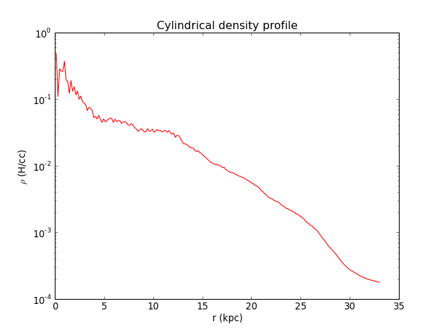
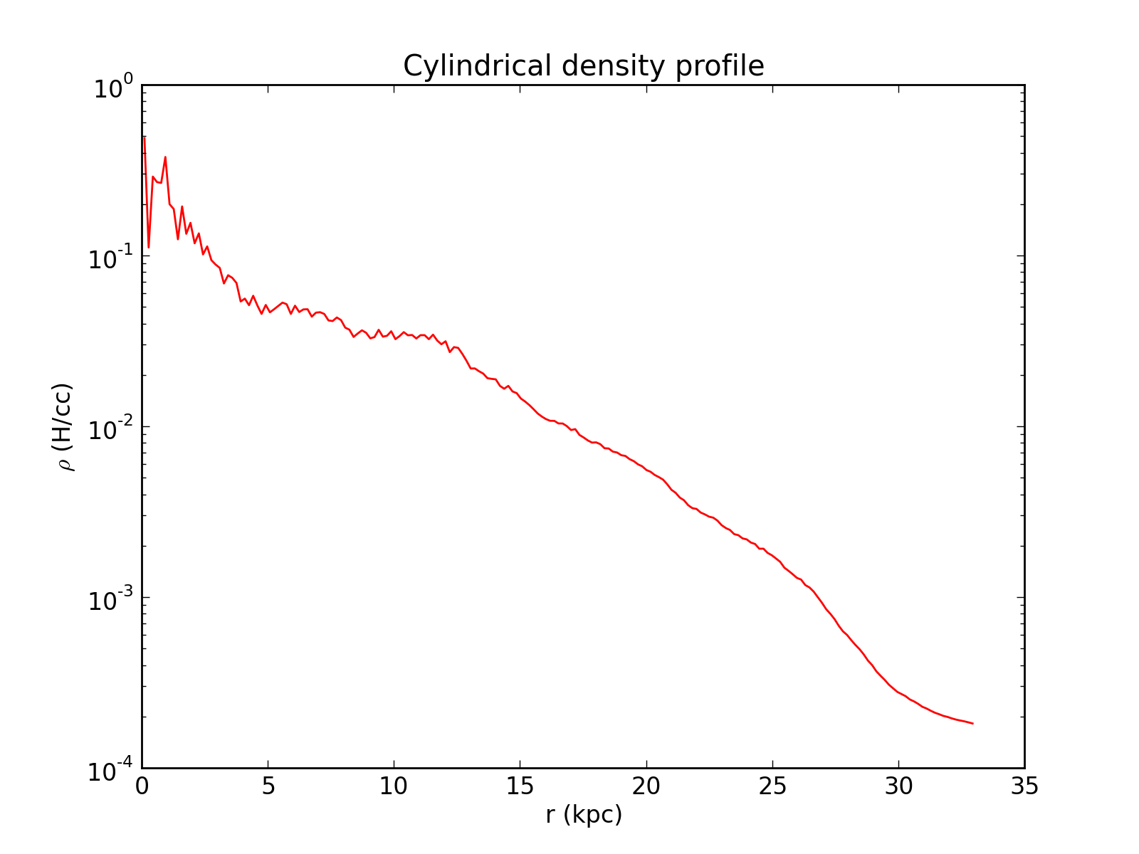
As we are interested in the density profile, we use the data field rho as the weight function. We also take 200 linearly spaced radial bins within the cylinder radius:

import numpy
rho_weight_func = lambda dset: dset["rho"]
r_bins = numpy.linspace(0.0, gal_radius, 200)

Now we compute the profile of the resulting PointDataset using the bin_cylindrical() function.

We set the divide_by_counts flag to True, because we’re averaging the density field in each cylindrical shell:

from pymses.analysis import bin_cylindrical
rho_profile = bin_cylindrical(point_dset, gal_center, gal_normal,\
    rho_weight_func, r_bins, divide_by_counts=True)

Finally, we can plot the profile with Matplotlib:

(Source code, png, hires.png, pdf)

Spherical profile of a set of particle data

Use case

You want to compute the spherical radial profile of a given particle data field.

Example : From a RAMSES cosmological simulation, you want to compute the radial density profile of a dark matter halo. You already know the position and the size of the halo.

We take the location and spatial extension of the dark matter halo to be:

halo_center = [ 0.567811, 0.586055, 0.559156 ]        # in box units
halo_radius = 0.00075                                 # in box units

Reading particle data from a RAMSES output

As already explained in Get a RAMSES output into PyMSES and Reading particles, we create the particle data source from the RAMSES output we are intersted in, reading only the mass and epoch fields:

from pymses import RamsesOutput
ro = RamsesOutput("/data/Aquarius/output", 193)
# Prepare to read the mass/epoch fields only
source = ro.particle_source(["mass", "epoch"])

Filtering all the initial particles within a given region of interest

See Data filtering for details.

Now we build the Sphere that will define the region of interest for the profile:

from pymses.utils.regions import Sphere
sph = Sphere(halo_center, halo_radius)

Then filter all the particles contained in the sphere by using a RegionFilter:

from pymses.filters import RegionFilter point_dset = RegionFilter(sph, source)

Filter all the particles which are initially present in the simulation using a PointFunctionFilter:

from pymses.filters import PointFunctionFilter
dm_filter = lambda dset: dset["epoch"] == 0.0
dm_parts = PointFunctionFilter(dm_filter, point_dset)

Computing the profile

As we are interested in the density profile, we use the data field mass as the weight function. We also take 200 linearly spaced radial bins within the sphere radius:

import numpy
m_weight_func = lambda dset: dset["mass"]
r_bins = numpy.linspace(0.0, halo_radius, 200)

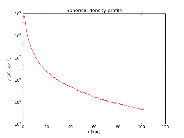
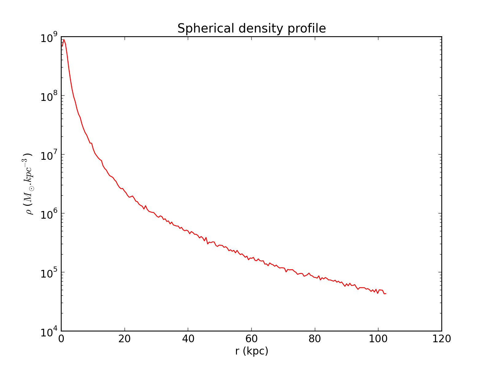
Now we compute the profile bin_spherical() function.

We set the divide_by_counts flag to False (optional, this is the default value), because we’re cumulating the masses of the particles in spherical shells:

from pymses.analysis import bin_spherical
# This triggers the actual reading of the particle data files from disk.
mass_profile = bin_spherical(dm_parts, halo_center, m_weight_func, r_bins, divide_by_counts=False)

To compute the density profile, we divide the mass profile by the volume of each spherical shell:

sph_vol = 4.0/3.0 * numpy.pi * r_bins**3
shell_vol = numpy.diff(sph_vol)
rho_profile = mass_profile / shell_vol

(Source code, png, hires.png, pdf)