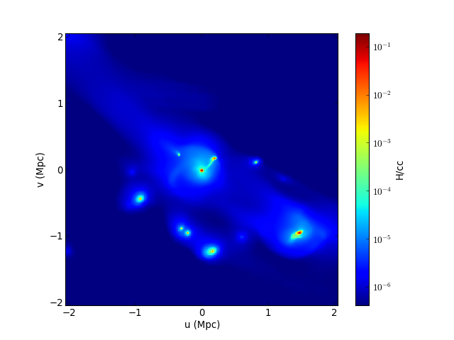
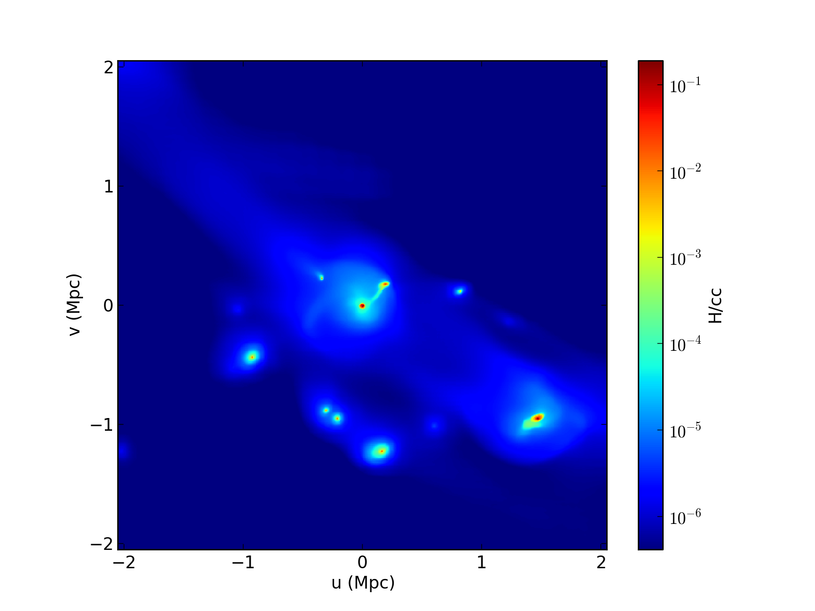
Ray-traced maps are computed in PyMSES by integrating a physical quantity along rays, each one corresponding to a pixel of the map. Ray-tracing is handled by a RayTracer. You can see two examples of this method below :
Important note on operators
You must keep in mind that any X Operator you use with this method must describe an intensive physical variable since this method compute an integral of an AMR quantity over each pixel surface and along the line-of-sight :
map[i,j] = \displaystyle\int_{z_{\text{min}}}^{z_{\text{max}}} X \textrm{d}S_{\text{pix}}\textrm{d}z
from numpy import array
import pylab
from pymses.analysis.visualization import *
from pymses import RamsesOutput
from pymses.utils import constants as C

# Ramses data
ioutput = 193
ro = RamsesOutput("/data/Aquarius/output/", ioutput)

# Map operator : mass-weighted density map
up_func = lambda dset: (dset["rho"]**2)
down_func = lambda dset: (dset["rho"])
scal_op = FractionOperator(up_func, down_func)

# Map region
center = [ 0.567811, 0.586055, 0.559156 ]
axes = {"los": array([ -0.172935, 0.977948, -0.117099 ])}

# Map processing
rt = raytracing.RayTracer(ro, ["rho"])
for axname, axis in axes.items():
	cam  = Camera(center=center, line_of_sight_axis=axis, up_vector="z", region_size=[3.0E-2, 3.0E-2], \
			distance=2.0E-2, far_cut_depth=2.0E-2, map_max_size=512)
	map = rt.process(scal_op, cam)
	factor = ro.info["unit_density"].express(C.H_cc)
	scale = ro.info["unit_length"].express(C.Mpc)

	# Save map into HDF5 file
	mapname = "gas_rt_mw_%s_%5.5i"%(axname, ioutput)
	h5fname = save_map_HDF5(map, cam, map_name=mapname)

	# Plot map into Matplotlib figure/PIL Image
	fig = save_HDF5_to_plot(h5fname, map_unit=("H/cc",factor), axis_unit=("Mpc", scale), cmap="jet")
#	pil_img = save_HDF5_to_img(h5fname, cmap="jet")

	# Save into PNG image file
#	save_HDF5_to_plot(h5fname, map_unit=("H/cc",factor), axis_unit=("Mpc", scale), img_path="./", cmap="jet")
#	save_HDF5_to_img(h5fname, img_path="./", cmap="jet")

#pylab.show()
(Source code, png, hires.png, pdf)
from numpy import array, zeros_like
import pylab
from pymses.analysis.visualization import *
from pymses import RamsesOutput
from pymses.utils import constants as C
# Ramses data
ioutput = 193
ro = RamsesOutput("/data/Aquarius/output/", ioutput)
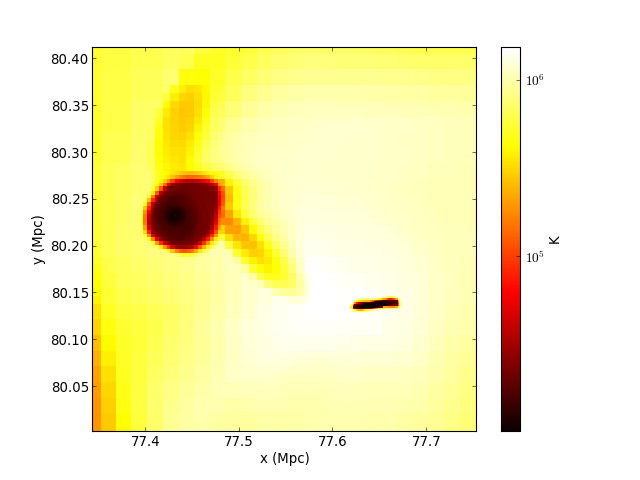
# Map operator : minimum temperature along line-of-sight
class MyTempOperator(Operator):
def __init__(self):
def invT_func(dset):
P = dset["P"]
rho = dset["rho"]
r = rho/P
# print r[(rho<=0.0)+(P<=0.0)]
# r[(rho<=0.0)*(P<=0.0)] = 0.0
return r
d = {"invTemp": invT_func}
Operator.__init__(self, d, is_max_alos=True)
def operation(self, int_dict):
map = int_dict.values()[0]
mask = (map == 0.0)
mask2 = map != 0.0
map[mask2] = 1.0 / map[mask2]
map[mask] = 0.0
return map
scal_op = MyTempOperator()
# Map region
center = [ 0.567111, 0.586555, 0.559156 ]
axes = {"los": "z"}
# Map processing
rt = raytracing.RayTracer(ro, ["rho", "P"])
for axname, axis in axes.items():
cam = Camera(center=center, line_of_sight_axis=axis, up_vector="y", region_size=[3.0E-3, 3.0E-3], \
distance=1.5E-3, far_cut_depth=1.5E-3, map_max_size=512)
map = rt.process(scal_op, cam)
factor = ro.info["unit_temperature"].express(C.K)
scale = ro.info["unit_length"].express(C.Mpc)
# Save map into HDF5 file
mapname = "gas_rt_Tmin_%s_%5.5i"%(axname, ioutput)
h5fname = save_map_HDF5(map, cam, map_name=mapname)
# Plot map into Matplotlib figure/PIL Image
fig = save_HDF5_to_plot(h5fname, map_unit=("K",factor), axis_unit=("Mpc", scale), cmap="hot", fraction=0.0)
# pil_img = save_HDF5_to_img(h5fname, cmap="hot")
# Save into PNG image file
# save_HDF5_to_plot(h5fname, map_unit=("K",factor), axis_unit=("Mpc", scale), img_path="./", cmap="hot")
# save_HDF5_to_img(h5fname, img_path="./", cmap="hot")
#pylab.show()
(Source code, png, hires.png, pdf)

from numpy import array
import pylab
from pymses.analysis.visualization import *
from pymses import RamsesOutput
from pymses.utils import constants as C
# Ramses data
ioutput = 193
ro = RamsesOutput("/data/Aquarius/output/", ioutput)
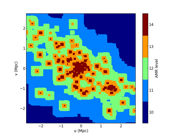
# Map operator : max. AMR level of refinement along the line-of-sight
scal_op = MaxLevelOperator()
# Map region
center = [ 0.567811, 0.586055, 0.559156 ]
axes = {"los": array([ -0.172935, 0.977948, -0.117099 ])}
# Map processing
rt = raytracing.RayTracer(ro, ["rho"])
for axname, axis in axes.items():
cam = Camera(center=center, line_of_sight_axis=axis, up_vector="z", region_size=[4.0E-2, 4.0E-2], \
distance=2.0E-2, far_cut_depth=2.0E-2, map_max_size=512, log_sensitive=False)
map = rt.process(scal_op, cam)
scale = ro.info["unit_length"].express(C.Mpc)
# Save map into HDF5 file
mapname = "gas_rt_lmax_%s_%5.5i"%(axname, ioutput)
h5fname = save_map_HDF5(map, cam, map_name=mapname)
# Plot map into Matplotlib figure/PIL Image
fig = save_HDF5_to_plot(h5fname, map_unit=("AMR level",1.0), axis_unit=("Mpc", scale), cmap="jet", discrete=True)
# pil_img = save_HDF5_to_img(h5fname, cmap="jet", discrete=True)
# Save into PNG image file
# save_HDF5_to_plot(h5fname, map_unit=("AMR level",1.0), axis_unit=("Mpc", scale), img_path="./", cmap="jet", discrete=True)
# save_HDF5_to_img(h5fname, img_path="./", cmap="jet", discrete=True)
#pylab.show()
(Source code, png, hires.png, pdf)

If you are using python 2.6 or higher, the RayTracer will try to use multiprocessing speed up. You can desactivate it to save RAM memory and processor use by setting the multiprocessing option to False:
map = rt.process(scal_op, cam, multiprocessing = False)