FFT-convolved maps

Intro

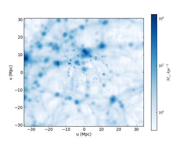
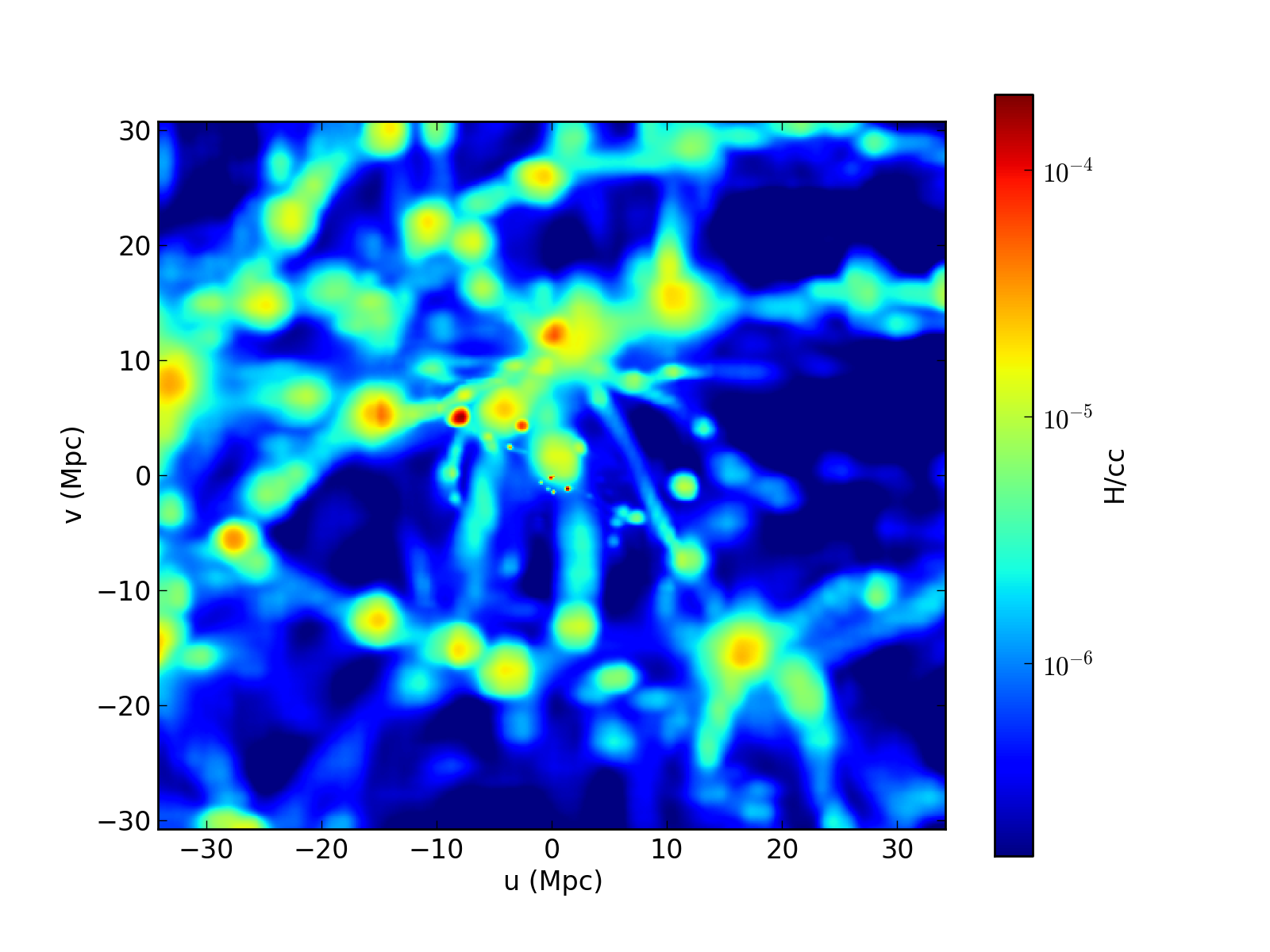
A very simple, fast and accurate data projection (3D->2D) method : each particle/AMR cell is convolved by a 2D gaussian kernel (Splatter) which size depends on the local AMR grid level.

The convolution of the binned particles/AMR cells histogram with the gaussian kernels is performed with FFT techniques by a MapFFTProcessor. You can see two examples of this method below :

• Particles map
• AMR data map

Important note on operators

You must keep in mind that any X Operator you use with this method must describe an extensive physical variable since this method compute a summation over particle/AMR quantities :

map[i,j] = \displaystyle\sum_{\text{particles/AMR cells}} X

Examples

Particles map

from numpy import array, log10
import pylab
from pymses.analysis.visualization import *
from pymses import RamsesOutput
from pymses.utils import constants as C

# Ramses data
ioutput = 193
ro = RamsesOutput("/data/Aquarius/output/", ioutput)
parts = ro.particle_source(["mass", "level"])

# Map operator : mass
scal_func = ScalarOperator(lambda dset: dset["mass"])

# Map region
center = [ 0.567811, 0.586055, 0.559156 ]
axes = {"los": array([ -0.172935, 0.977948, -0.117099 ])}

# Map processing
mp = fft_projection.MapFFTProcessor(parts, ro.info)
for axname, axis in axes.items():
	cam  = Camera(center=center, line_of_sight_axis=axis, up_vector="z", region_size=[5.0E-1, 4.5E-1], \
			distance=2.0E-1, far_cut_depth=2.0E-1, map_max_size=512)
	map = mp.process(scal_func, cam, surf_qty=True)
	factor = (ro.info["unit_mass"]/ro.info["unit_length"]**2).express(C.Msun/C.kpc**2)
	scale = ro.info["unit_length"].express(C.Mpc)

#	pylab.imshow(map)
#	pylab.show()
	# Save map into HDF5 file
	mapname = "DM_Sigma_%s_%5.5i"%(axname, ioutput)
	h5fname = save_map_HDF5(map, cam, map_name=mapname)

	# Plot map into Matplotlib figure/PIL Image
	fig = save_HDF5_to_plot(h5fname, map_unit=("$M_{\odot}.kpc^{-2}$",factor), axis_unit=("Mpc", scale), cmap="Blues", fraction=0.1)
#	pil_img = save_HDF5_to_img(h5fname, cmap="Blues", fraction=0.1)

	# Save map into PNG image file
#	save_HDF5_to_plot(h5fname, map_unit=("$M_{\odot}.kpc^{-2}$",factor), \
#			axis_unit=("Mpc", scale), img_path="./", cmap="Blues", fraction=0.1)
#	save_HDF5_to_img(h5fname, img_path="./", cmap="Blues", fraction=0.1)

# pylab.show()

(Source code, png, hires.png, pdf)

AMR data map

from numpy import array
import pylab
from pymses.analysis.visualization import *
from pymses import RamsesOutput
from pymses.utils import constants as C

# Ramses data
ioutput = 193
ro = RamsesOutput("/data/Aquarius/output/", ioutput)
amr = ro.amr_source(["rho", "P"])

# Map operator : mass-weighted density map
up_func = lambda dset: (dset["rho"]**2 * dset.get_sizes()**3)
down_func = lambda dset: (dset["rho"] * dset.get_sizes()**3)
scal_func = FractionOperator(up_func, down_func)

# Map region
center = [ 0.567811, 0.586055, 0.559156 ]
axes = {"los": array([ -0.172935, 0.977948, -0.117099 ])}

# Map processing
mp = fft_projection.MapFFTProcessor(amr, ro.info)
for axname, axis in axes.items():
	cam  = Camera(center=center, line_of_sight_axis=axis, up_vector="z", region_size=[5.0E-1, 4.5E-1], \
			distance=2.0E-1, far_cut_depth=2.0E-1, map_max_size=512)
	map = mp.process(scal_func, cam)
	factor = ro.info["unit_density"].express(C.H_cc)
	scale = ro.info["unit_length"].express(C.Mpc)

#	pylab.imshow(map)
	# Save map into HDF5 file
	mapname = "gas_mw_%s_%5.5i"%(axname, ioutput)
	h5fname = save_map_HDF5(map, cam, map_name=mapname)

	# Plot map into Matplotlib figure/PIL Image
	fig = save_HDF5_to_plot(h5fname, map_unit=("H/cc",factor), axis_unit=("Mpc", scale), cmap="jet")
#	pil_img = save_HDF5_to_img(h5fname, cmap="jet")

	# Save into PNG image file
#	save_HDF5_to_plot(h5fname, map_unit=("H/cc",factor), axis_unit=("Mpc", scale), img_path="./", cmap="jet")
#	save_HDF5_to_img(h5fname, img_path="./", cmap="jet")

# pylab.show()

(Source code, png, hires.png, pdf)